JHU Open Source GIS with Isaacs
Ref: Dr. Rachel Isaacs (2019). Open Source GIS. JHU Course AS.420.703.81. Email: risaacs6@jhu.edu
_______________________________________________________________________
Summary
An overview of the fundamentals of mapping, photogrammetry, geographic information science, and remote sensing.
Programs: QGIS (https://www.qgis.org/en/site/), Google Earth Engine (GEE), & R.


__________________________________________________________________________________
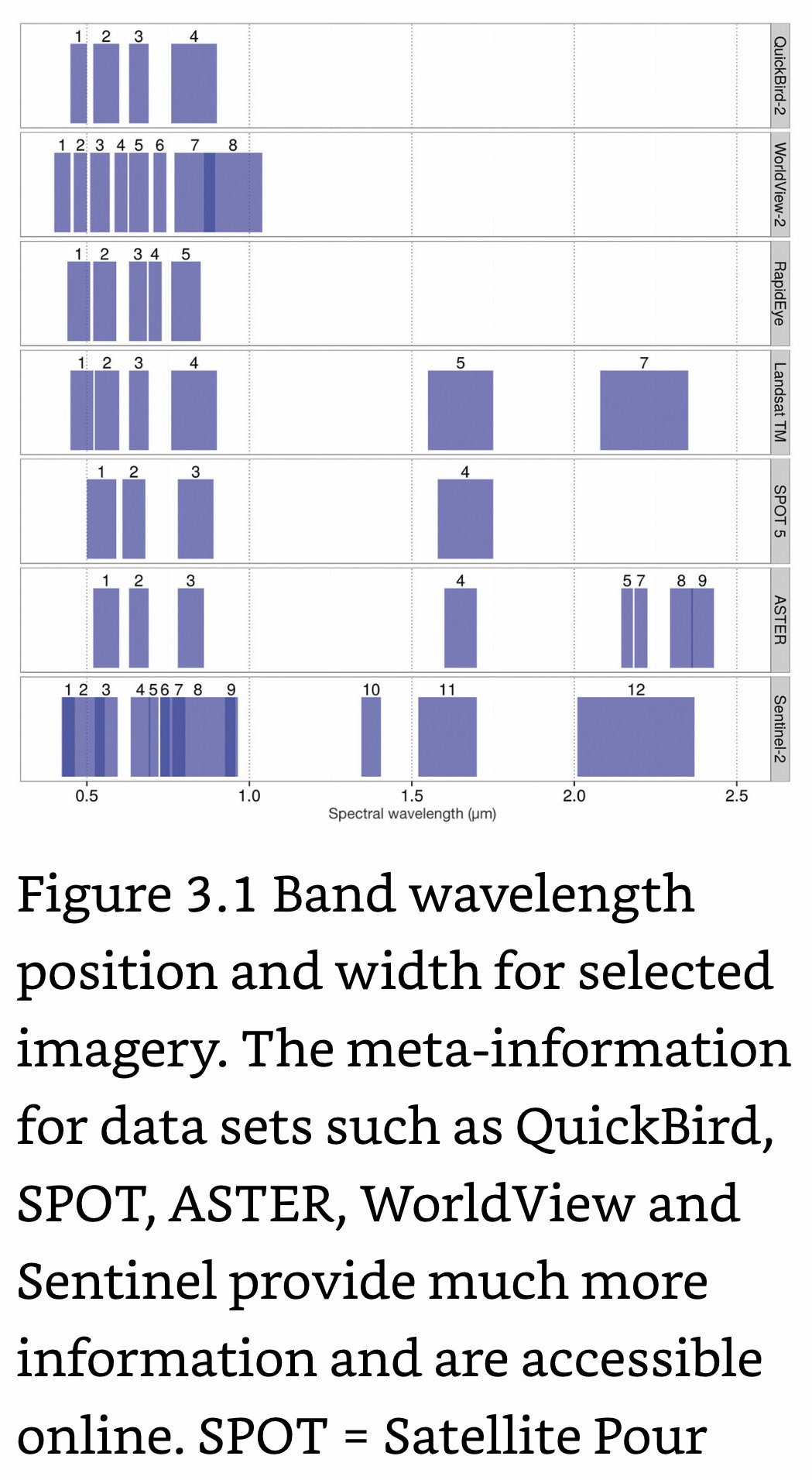
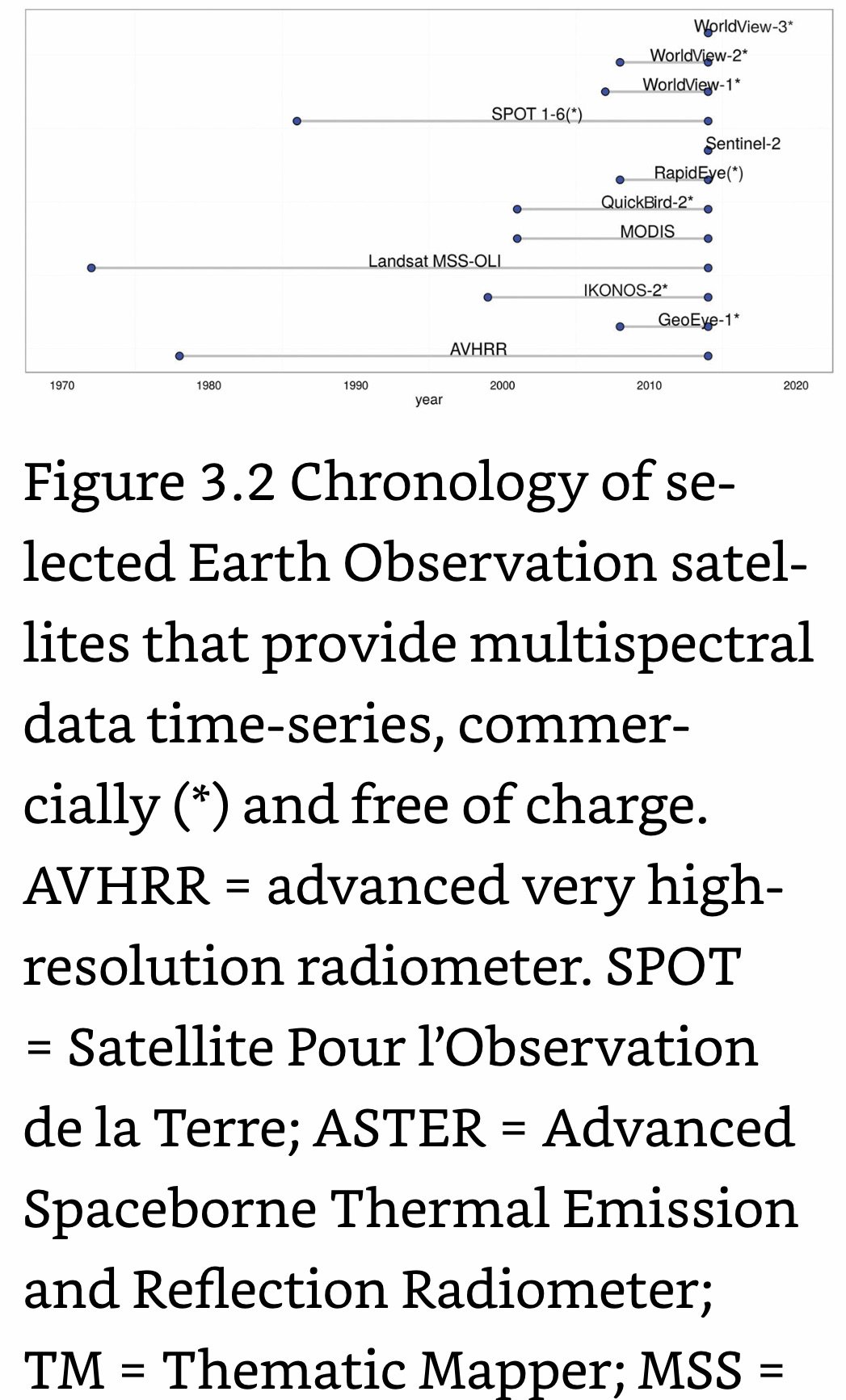
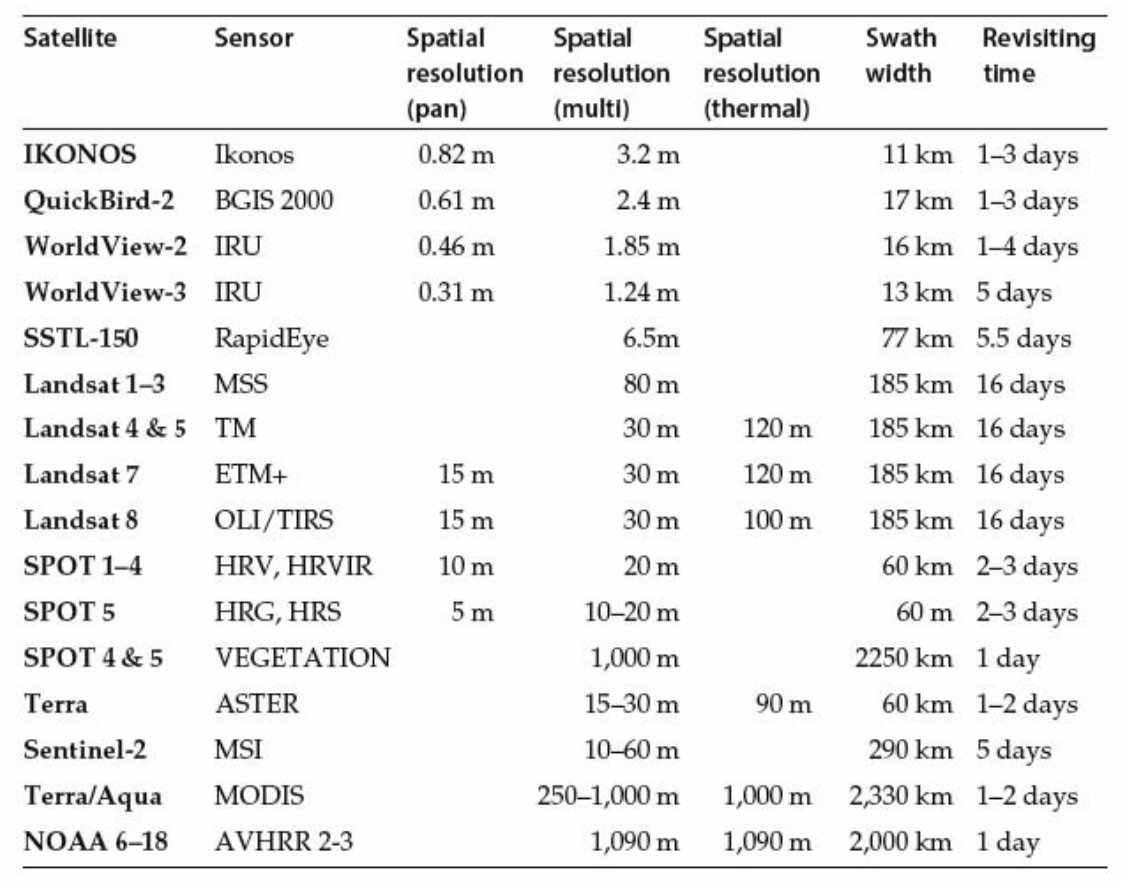
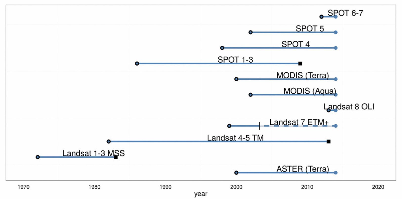
Landsat Satellite Missions
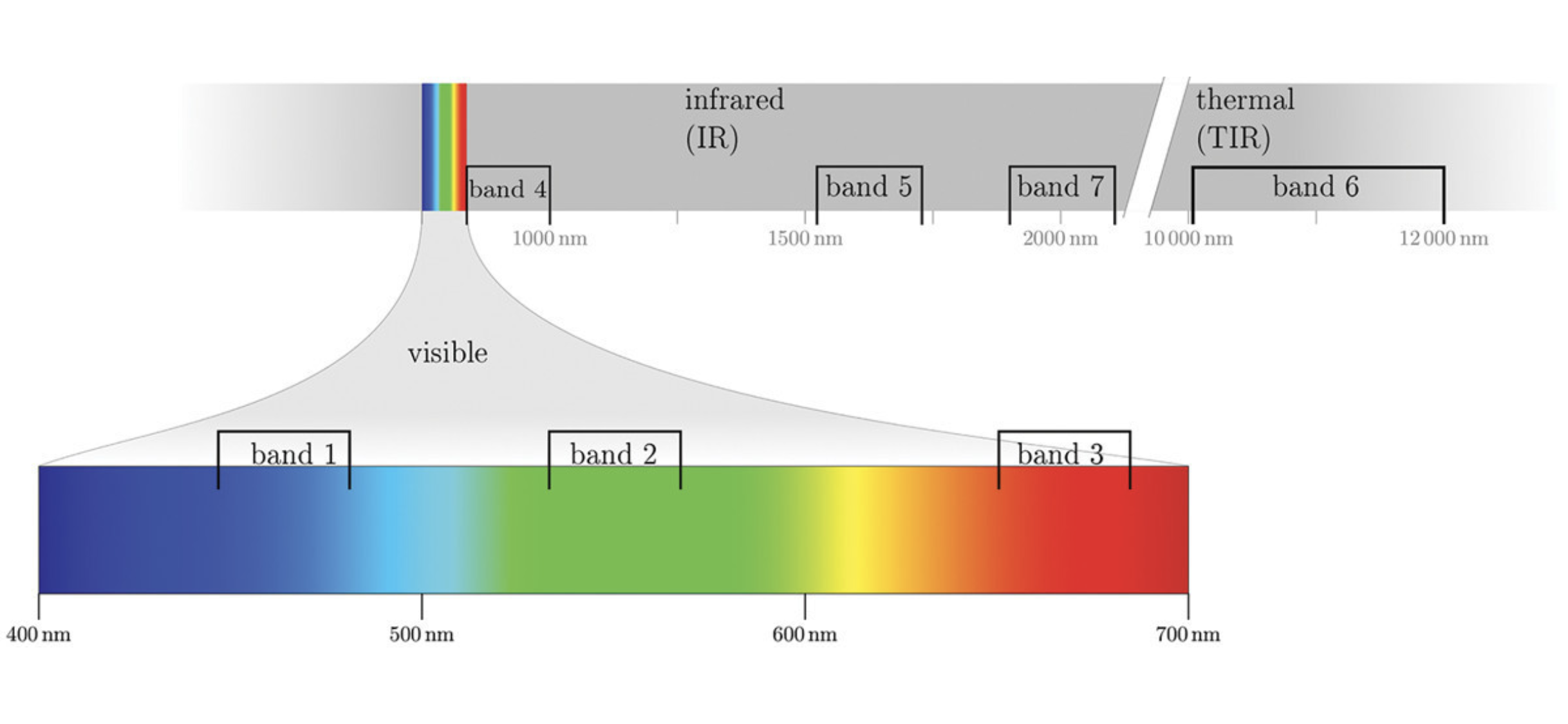
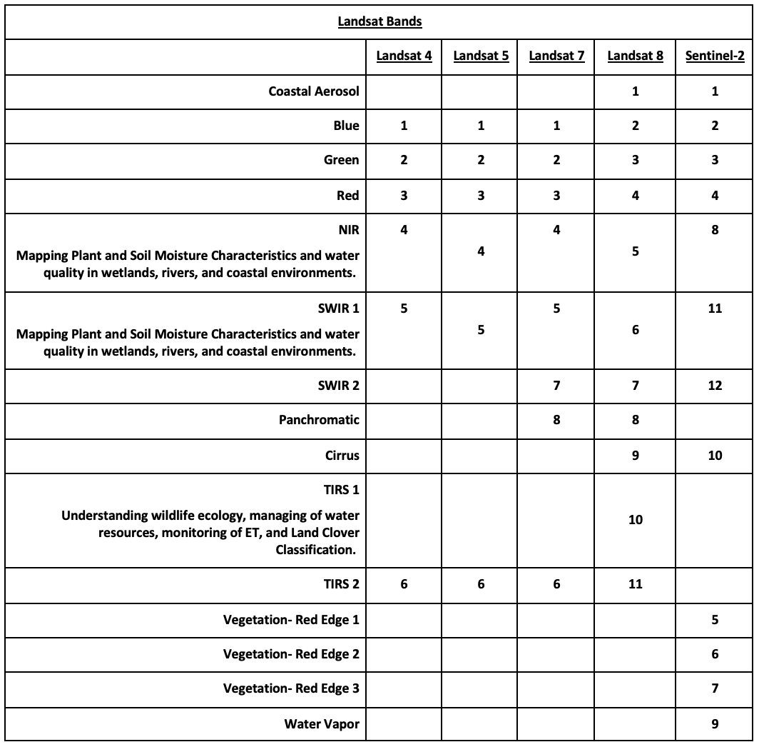
Landsat Group 1 (LS 1-3): Equipped with Multispectral Scanner (MSS), which recorded data in 4 spectral bands; two visible and two near-IR (NIR).
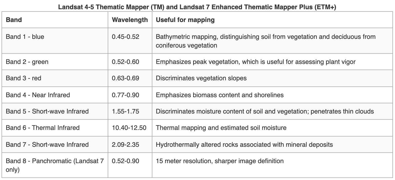
Landsat Group 2 (LS 4-7): Equipped with Thematic Mapper (TM) or Enhanced Thematic Mapper (ETM+) with finer resolution size, expanded spectral coverage, additional bands in the middle- IR (MIR aka SWIR- short wave IR) and thermal IR wavelengths.
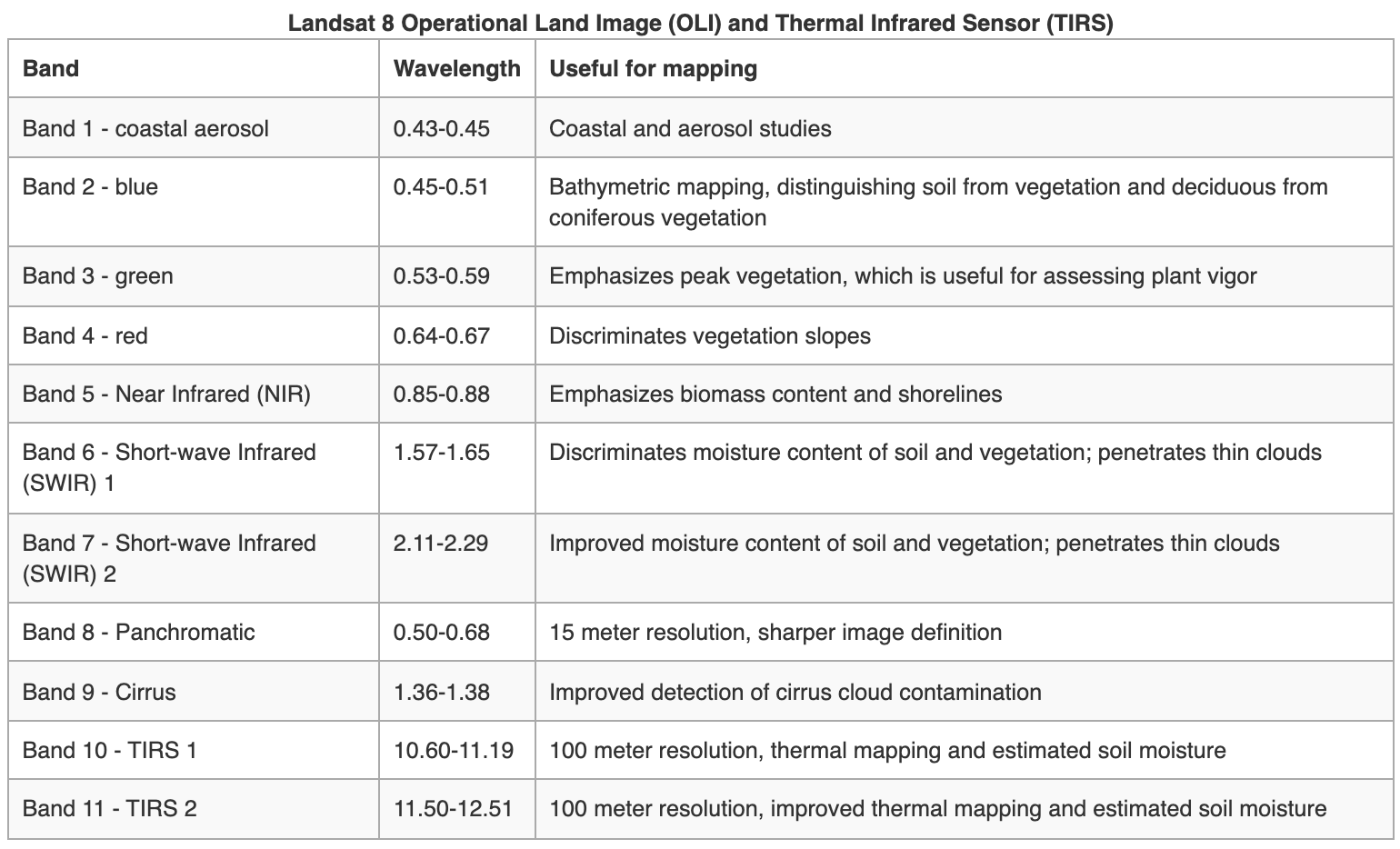
Landsat Group 3 (LS 8-9): Equipped with an operational land imager (OLI) and Thermal IR Sensor (TIRS). The OLI augments the TM with the addition of a deep blue and a cirrus band, while TIRS adds a second thermal band.
Landsat 9 is scheduled for launch in Sep, 2021.
NASA builds and launches the satellites while the USGS Operates the Missions.


__________________________________________________________________________________
---QGIS How To---
__________________________________________________________________________________
Image Classification
Image Classification: The process of sorting pixels into a finite number of individual classes, or categories of data, based on their spectral response (the measured brightness of a pixel across the image bands, as reflected by the pixel’s spectral signature).
Supervised: Uses image pixels representing regions of known, homogenous surface composition -- training areas -- to classify unknown pixels.
Determine a classification scheme
Create training areas
Digitizing: Drawing Polygons around areas in an image.
Seeding: Grows areas based on spectral similarity to seed pixel.
Generate training area signatures
Evaluate and refine signatures
Assign pixels to classes using a classifier (a.k.a., “decision rule”).
Parametric: Image is classified based on a statistical representation of the data derived from the training area signatures; all image pixels are classified.
Minimum Distance: Classifies pixels based on the spectral distance between the candidate pixel and the mean value of each signature (class) in each image band.
Maximum Likelihood: Classifies pixels based on the probability that a pixel falls within a certain class.
Non-parametric: Pixels are classified as objects in feature space; only those pixels within the feature space object are classified.
Parallelepiped: The pixels values are compared to upper and lower limits of each signature class (i.e., the min/max pixel values in each band, or the mean of each band +/- 2 standard deviations)
Feature Space: Classifies pixels that fall within non-parametric signatures identified in the feature space image not used very often because it is difficult to accurately create and evaluate non-parametric signatures.
Unsupervised (aka clustering): Identifies and assigns groups of pixels exhibiting a similar spectral response a meaning (i.e. a land-cover categorization).
Determine a general classification scheme
Group pixels into groups of similar values based on pixel- value relationships (i.e. Iterative ISODATA technique).
Iterative Self-Organizing Data Analysis (ISODATA) Technique: Uses “spectral distance” between image pixels in feature space to classify pixels into a specified number of unique spectral groups (or “clusters”).
Assign spectral classes to informational classes.
__________________________________________________________________________________
Vegetation Indices
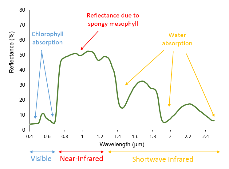
Vegetation Indexes (VI): Vegetation reflects strongly in the NIR and weakly in the SWIR portions of the EM Spectrum.
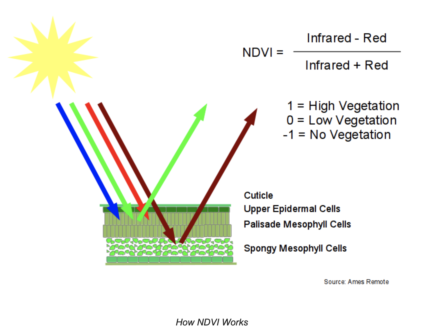
Normalized Difference Vegetation Index (NDVI): Quantifies vegetation by measuring the difference between NIR (which chlorophyl vegetation reflects) and red light (which vegetation absorbs); NDVI = (NIR - Red) / (NIR + Red)
NDVI is based on the observation that green plants reflect infrared light (to avoid overheating), but absorb visible light (to power photosynthesis). This gives green plants a light reflection signature that can distinguish them from objects that absorb all spectra of light or different spectra of light from plants.
NDVI ranges from -1 (unhealthy) to 1 (healthy).
Delta/Differenced NDVI (dNDVI): dNDVI = preNDVI – postNDVI
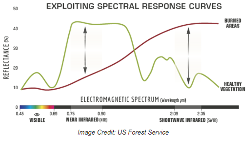
Normalized Burn Ratio (NBR): Highlight burned areas and estimate fire severity; NBR= (NIR-SWIR)/(NIR+SWIR)
Delta/Differenced NBR (dNBR): Assesses the amount of vegetation and soil changes resulting from fire; dNBR = preNBR – postNBR
Normalized Difference Snow Index (NDSI): Estimates the amount of a pixel covered in snow; NDSI = (Green – SWIR) / (Green + SWIR)
Normalized Difference Water Index (NDWI): Delineates open water features, enhancing their presence in SRS; NDWI = (G - NIR) / (G + NIR)
Normalized Pigment Chlorophyll Ratio Index (NPCRI): Numerical indicator used to determine crop and/or vegetation clorphyll content; NPCRI = (Red – Blue) / (Red + Blue)
Normalized Difference Glacier Index (NDGI): Used to detect and monitor glaciers; NDGI = (NIR – Green) / (NIR + Green)
Normalized Different Moisture Index (NDMI): Used in combination with NDVI and/or ADVI to calculate vegetation moisture; NDMI = (NIR – SWIR) / (NIR + SWIR)
Advanced Vegetation Index (AVI): Similar to NDVI, monitors crop and forest variations over time; AVI = (NIR * (1 – Red) * (NIR – Red))1/3
Bare Soil Index (BSI): Combines Blue, Red, NIR, and SWIR to capture soil variations; BSI = ((Red+SWIR) - (NIR+Blue)) / ((Red+SWIR) + (NIR+Blue))
Topographic Wetness Index (TWI): TWI= In (upslope contributing area/tan(slope)) in dry- wet.
__________________________________________________________________________________
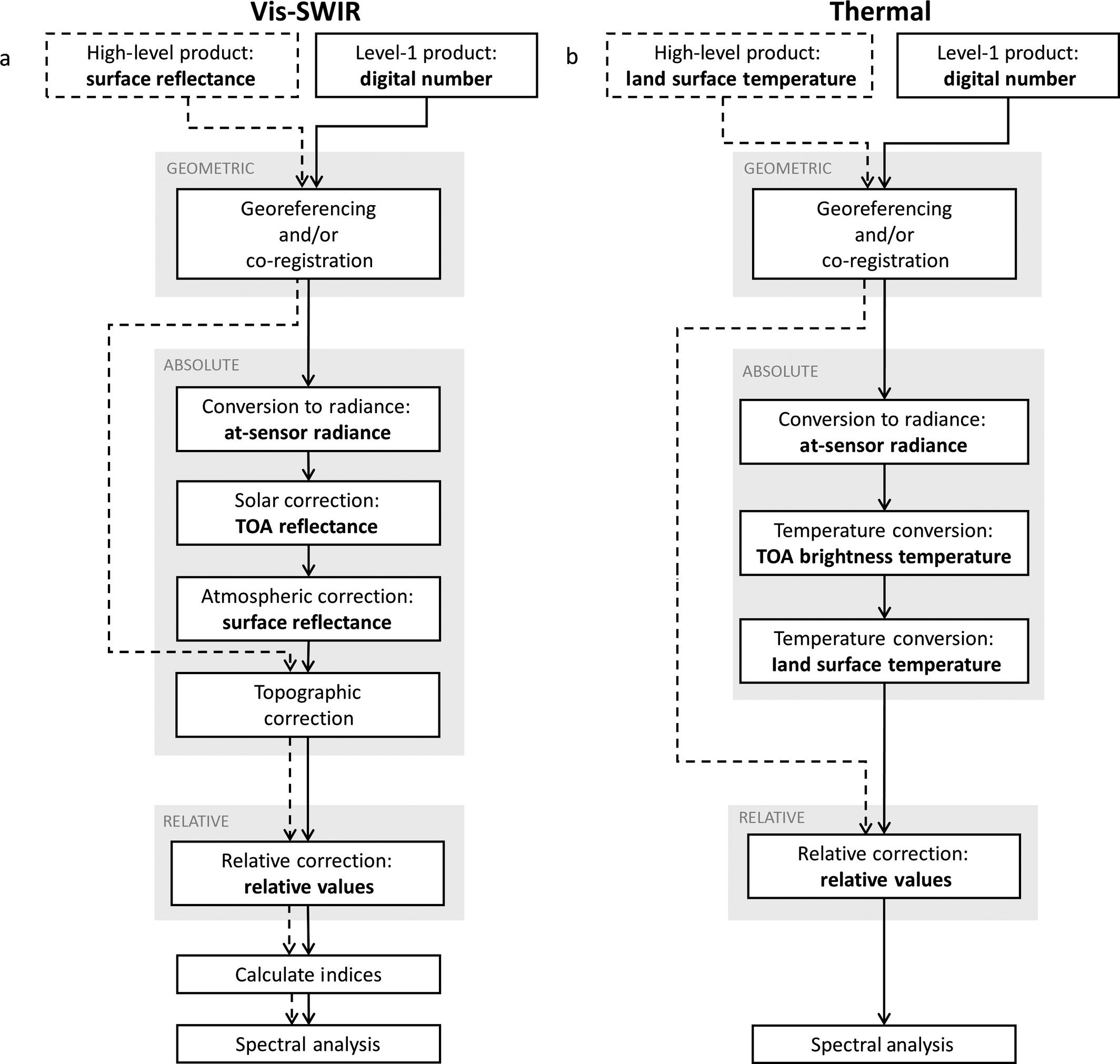
Pre-Processing Steps
Geometric Correction: Exact positioning of the image.
Georeferencing: Alignment of imagery to geographic location
Orthorectifying: Correction for the effects of relief and view direction on pixel location.
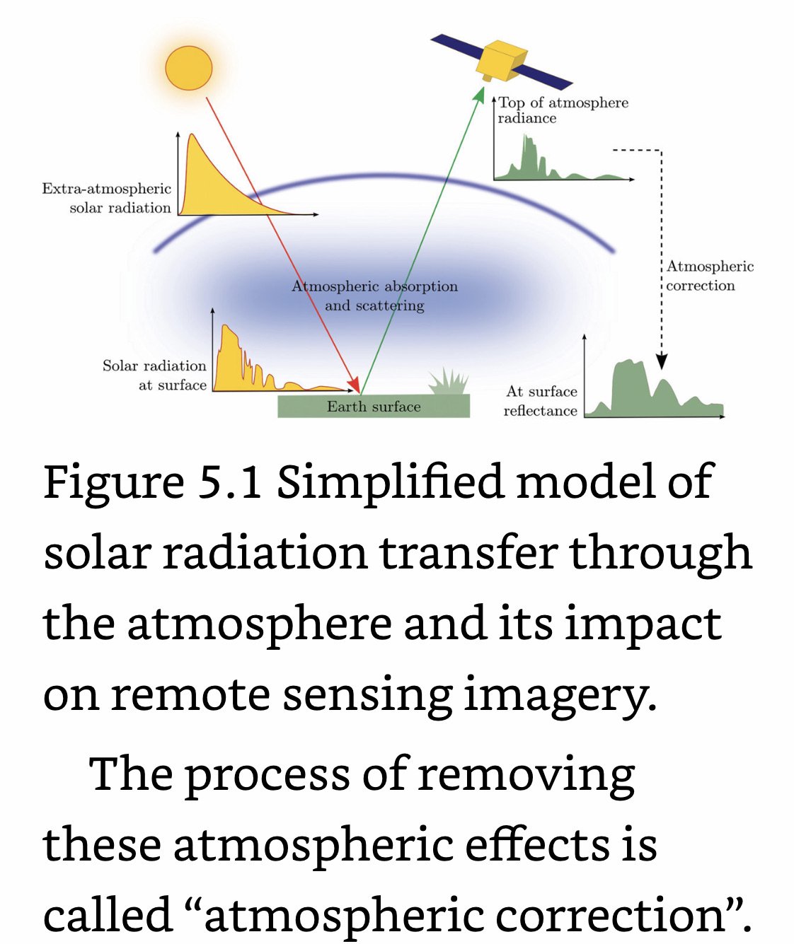
Absolute Radiometric Correction (aka Absolute correction): Account for sensor, solar, atmospheric, and topographic effects.
Conversion to Radiance
Solar Correction: Accounts for solar influences on pixel values. Solar corrections converts at-sensor radiance to top of atmosphere (TOA) reflectance by incorporating exo-atmospheric solar irradiance (power of the sun), earth distance, and solar elevation angle.
Atmospheric Correction: Accounts for scattering and absorption in the Earth’s atmosphere.
Topographic Correction: Accounts for illumination effects from slope, aspect, and elevation.
Relative Radiometric Correction: Brings each band of an image to the same radiometric scale as the corresponding band of a referenced image to account for sensor, solar, and atmospheric differences.
__________________________________________________________________________________
Terrain Analysis
Add a DEM
Add Hillshade
Raster- Analysis- Hillshade
Input DEM, change Azimuth if you want, add an output layer in save file.
Change DEM Coloring
Go to DEM Layer- Symbology- color ramp- elevation green-brown-white. Change Transparency (60%).
Slope
Go to Raster- Analysis- Slope
Input DEM Layer, Save as a slope file.
Change Symbology: Color Ramp- Green-Red-Yellow (shows high slopes). Change Transparency (60%) to make more visible.
Aspect
Go to Raster- Analysis- Aspect
Input DEM Layer, Return 0 for flight, save as aspect file.
Change Symbology: Single Band Single Pseudocolor- Color Ramp- 8 Classes: Inferno
_______________________________________________________________________
Adding Lat/Long to a Map
Layer- Add Layer- Add delimited text layer.
Browse to the file with your data. Make sure that csv is selected for File format. Additionally, make sure that X field represents the column for your longitude points and Y field for latitude. QGIS is smart enough to recognize longitude and latitude columns but double check!
Select your CRS.
_______________________________________________________________________
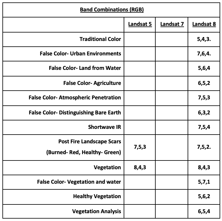
Creating a Multi-Band Image (Combining Spectral Data)
Open Raster- Build Virtual Raster.
Add all Bands and Run.
_______________________________________________________________________
Vector Geoprocessing
Clip: Clipping Data to create a new shape file.
Add Input Layer, Clip Layer, and name output file.
Area Calculation
Open Field Calculator in attribute table in editing mode.
Create a new field- name output field name- name outfield field type ($Area= sqm).
_______________________________________________________________________
Creating a Shapefile from a CSV
Go to Layer- Add Layer- Add Delimited Text Layer.
Ensure Coordinates on CSV align with X-field and Y-field and set CRS.
Add to Map.
Export and save as a shape file.
_______________________________________________________________________
Re-Project Data to Match CRS
Go to vector menu- Data management tools- Reproject Layer.
_______________________________________________________________________
---GEE How To---
Google Earth Engine Tutorial: https://courses.spatialthoughts.com/end-to-end-gee.html
Google Earth Python Mapping: https://geemap.org/
GIS Courses (GEE for Agrohydrology, Drone Imagery Processing, Hydrology): https://courses.gisopencourseware.org//
_______________________________________________________________________
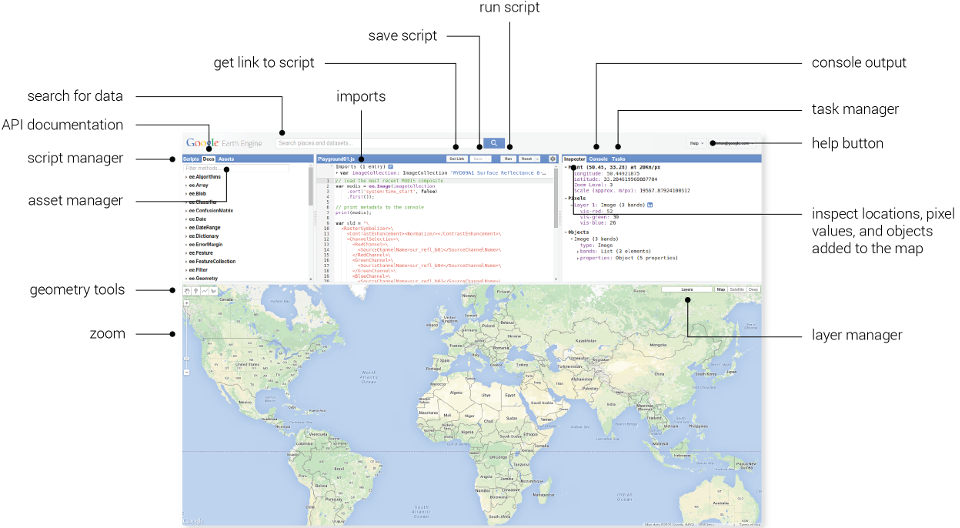
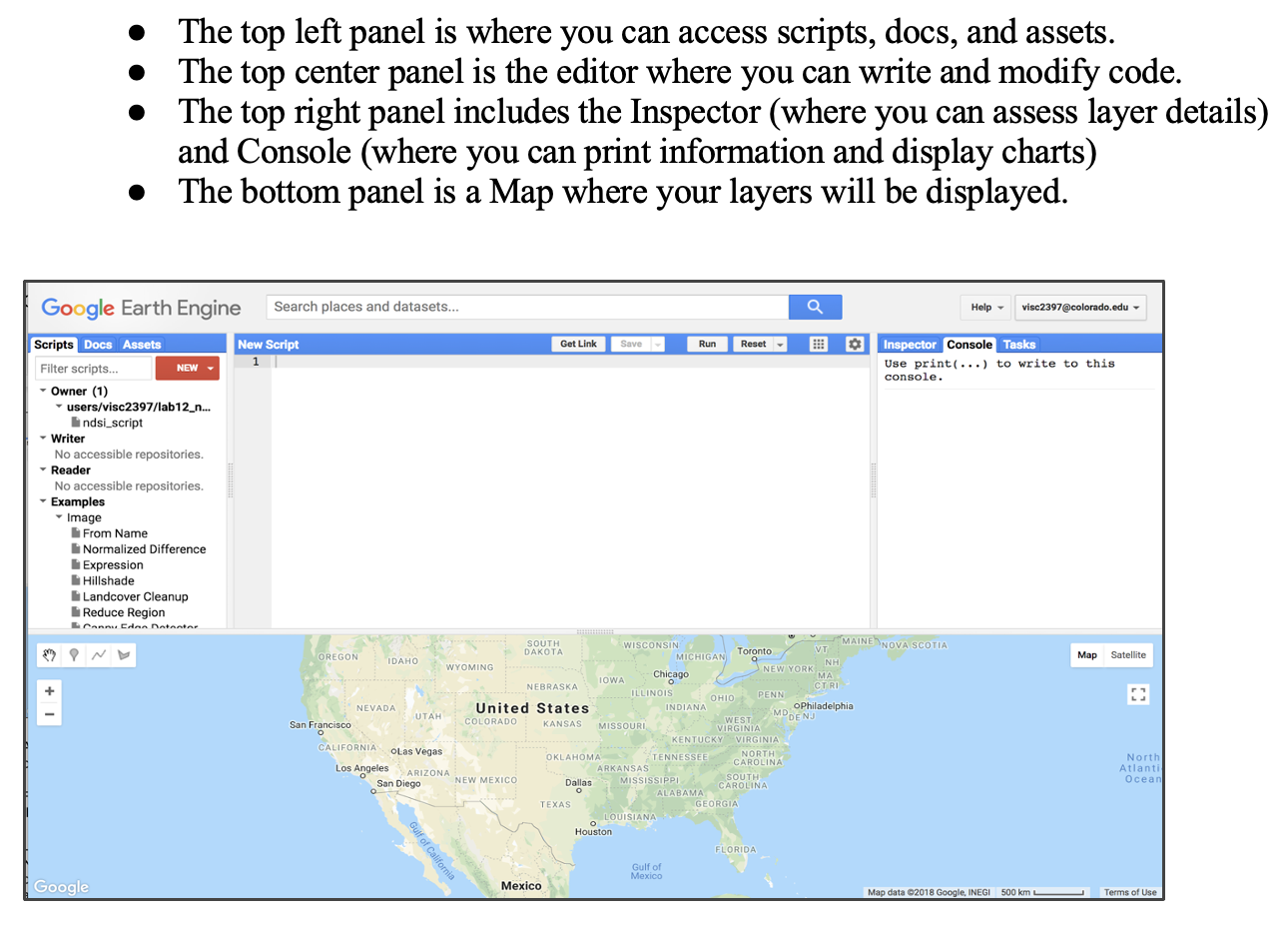
Google Earth Engine
Open GEE.
Add VI Code you want to conduct.
Search and pin a location.
Search and pin a GIS Image Set.
Run VI Program.
_______________________________________________________________________
---R---
R Toolboxes: http://book.ecosens.org/software/rstoolbox/
Simple Features for R: https://cran.r-project.org/web/packages/sf/vignettes/sf1.html
Find R packages with keywords (findPackage function from packagefinder): https://www.zuckarelli.de/packagefinder/tutorial.html
_______________________________________________________________________
Adding a Country Shapefile
Clear memory: rm(list=ls())
Set Working Directory: setwd("~/Desktop/GIS Open Source/Activity 4")
Install requisite packages:
install.packages("sf")
install.packages("terra")
install.packages("plotwidgets")
install.packages("ggshadow")
install.packages("ggspatial")
install.packages("ggnewscale")
install.packages("janitor")
install.packages("tidyverse")
install.packages("rgdal")
Load all packages
library(raster)
library(terra)
library(sf)
library(tidyverse)
library(plotwidgets)
library(ggshadow)
library(ggspatial)
library(ggnewscale)
library(janitor)
library(rgdal)
install.packages("devtools")
Load Country
World_Countries_Generalized <- "World_Countries__Generalized_"
limits <- readOGR(dsn = ".", layer = "World_Countries_Generalized")
limits <- ne_countries(scale = 50, returnclass = "sf")
_______________________________________________________________________
Unsupervised Kmeans Classification
Create a stack with all of our bands
Clear memory: rm(list=ls())
Add Bands
blue = raster("LT05_L1TP_166039_19950929_20181025_01_T1_B1.tif")
green = raster("LT05_L1TP_166039_19950929_20181025_01_T1_B2.tif")
red = raster("LT05_L1TP_166039_19950929_20181025_01_T1_B3.tif")
nir = raster("LT05_L1TP_166039_19950929_20181025_01_T1_B4.tif")
swir1 = raster("LT05_L1TP_166039_19950929_20181025_01_T1_B5.tif")
swir2 = raster("LT05_L1TP_166039_19950929_20181025_01_T1_B7.tif")
land5_stack = stack(blue, green, red, nir, swir1, swir2)
land5_matrix <- getValues(land5_stack)
i <- which(!is.na(land5_matrix))
land5_matrix <- na.omit(land5_matrix)
set.seed(99)
# This code converts a sample to a matrix and this random sample will be used to train and test the data:
land5_matrix2 <-land5_matrix[sample(nrow(land5_matrix), 500),]
rfl5 = randomForest(land5_matrix2)
rf_proxl8 <- randomForest(land8_matrix2,ntree = 1000, proximity = TRUE)$proximity
Install requisite packages:
install.packages("sp")
install.packages("raster")
install.packages("rgdal")
install.packages("RColorBrewer")
install.packages("ggplot2")
library(raster)
library(rgdal)
library(ggplot2)
## The "5" in this case refers to the number of clusters you want to create
l8_rf <- kmeans(rf_proxl8, 5, iter.max = 100, nstart = 10)
land8_rf <- randomForest(land8_matrix2,as.factor(l8_rf$cluster),ntree = 500)
l8_rf_raster<- predict(land8_stack,land8_rf)
plot(l8_rf_raster)
kmnclusterl5 <- kmeans(land5_matrix, centers = 5, iter.max = 100, nstart = 5, algorithm="Lloyd")
kmeans_rasterl8 <- raster(land8_stack)
kmeans_rasterl8[i] <- kmnclusterl8$cluster
plot(kmeans_rasterl8)
writeRaster(x = kmeans_rasterl8,
filename="~/Desktop/GIS Open Source/Activity 8/kmeansl8.tif",
format = "GTiff", # save as a tif
overwrite = TRUE) # OPTIONAL - be careful. This will OVERWRITE previous files.
_______________________________________________________________________
Load and View Multispectral Data
### Clear memory: rm(list=ls())
# Install packages (if necessary) and load your package library
# You NEED to load a package library every time
# To check that a package is active, click on the Packages tab to the right and
# sp automatically loads with the raster package
#install.packages("sp")
#install.packages("raster")
#install.packages("rgdal")
install.packages("RColorBrewer")
install.packages("ggplot2")
library(raster)
library(rgdal)
library(ggplot2)
##### There are three different Raster structures that you choose from depending on how many bands you need for a scene.
## RasterLayer = one file, one band
## RasterBrick = one file, multiple bands. Commonly used with RGB images
## RasterStack = multiple files, multiple bands (Landsat GeoTIFFs)
####### IMPORT MULTISPECTRAL DATA #################
### Download data from https://earthexplorer.usgs.gov/
### Once you have downloaded the data, unzip it on your computer and save it to a working folder
## Remember you should see all of your individual bands
##### Set your working directory using one of the methods learned to the folder where your bands are locate
### To note, you can set your working directory multiple times in a session
## If you want to load your bands individually, you create a raster stack
## Set each band name as an object attached to its associated raster
blue = raster("clipped_LC08_L1TP_172039_20190520_20190604_01_T1_B2.tif")
green = raster("clipped_LC08_L1TP_172039_20190520_20190604_01_T1_B3.tif")
red = raster("clipped_LC08_L1TP_172039_20190520_20190604_01_T1_B4.tif")
nir = raster("clipped_LC08_L1TP_172039_20190520_20190604_01_T1_B5.tif")
swir1 = raster("clipped_LC08_L1TP_172039_20190520_20190604_01_T1_B6.tif")
swir2 = raster("clipped_LC08_L1TP_172039_20190520_20190604_01_T1_B7.tif")
## Create an image using three bands and place them in the rgb channels
# example r=swir1
blue = raster("Clipped_LS8_VirtualLC08_L1TP_172039_20210626_20210707_01_T1_B2.tif")
nir = raster("Clipped_LS8_VirtualLC08_L1TP_172039_20210626_20210707_01_T1_B5.tif")
swir1 = raster("Clipped_LS8_VirtualLC08_L1TP_172039_20210626_20210707_01_T1_B6.tif")
rgb = stack(swir1, nir, blue) #chosen to emphasize vegetation
# Plot the image stack you just created using a linear stretch so the image isn't so washed out
# Look at the raster package for this function to see other types of stretches
plotRGB(rgb, stretch='lin')
## Though we are plotting a 3-band image, you can also plot each band individually
plot(blue)
e <- extent(229185, 345195, 4383585, 4472265)
# Crop the red band based on the exten
redcrop <- crop(red, e)
# Plot the cropped data to make sure everything worked properly
plot(redcrop)
# Crop the near infrared band based on the extent
nircrop <- crop(nir, e)
# Plot the cropped data to make sure everything worked properly
plot(nircrop)
_______________________________________________________________________
Perform Unsupervised Classification
#### METHOD 1: KMEANS ####
## This method clusters observations into a chosen number of categories based on the mean spectral signature.
## The algorithm is looking for clusters with similar spectral signatures (e.g. water)
### First, let's create a stack with all of our bands
land8_stack = stack(blue, green, red, nir, swir1, swir2)
blue = raster("Clipped_LS8_VirtualLC08_L1TP_172039_20210626_20210707_01_T1_B2.tif")
green = raster("Clipped_LS8_VirtualLC08_L1TP_172039_20210626_20210707_01_T1_B2.tif")
red = raster("Clipped_LS8_VirtualLC08_L1TP_172039_20210626_20210707_01_T1_B3.tif")
nir = raster("Clipped_LS8_VirtualLC08_L1TP_172039_20210626_20210707_01_T1_B4.tif")
swir1 = raster("Clipped_LS8_VirtualLC08_L1TP_172039_20210626_20210707_01_T1_B5.tif")
swir2 = raster("Clipped_LS8_VirtualLC08_L1TP_172039_20210626_20210707_01_T1_B6.tif")
land8_stack = stack(blue, green, red, nir, swir1, swir2)
### Before we can perform a classification, we need to convert the raster dataset to a matrix (array)
# We will also remove any pixels from the analysis containing NA values
land8_matrix <- getValues(land8_stack)
i <- which(!is.na(land8_matrix))
land8_matrix <- na.omit(land8_matrix)
# It is important to set the seed generator because `kmeans` initiates the centers in random locations
set.seed(99)
# We want to create 5 clusters, allow 500 iterations, start with 5 random sets using "Lloyd" method
## Centers refers to the number of clusters you want to create
kmnclusterl8 <- kmeans(land8_matrix, centers = 5, iter.max = 100, nstart = 5, algorithm="Lloyd")
# We need to convert the kmeans cluster analysis back to a raster layer
kmeans_rasterl8 <- raster(land8_stack)
kmeans_rasterl8[i] <- kmnclusterl8$cluster
plot(kmeans_rasterl8)
writeRaster(x = kmeans_rasterl8,
filename="~/Desktop/GIS Open Source/Activity 8/kmeansl8.tif",
format = "GTiff", # save as a tif
overwrite = TRUE) # OPTIONAL - be careful. This will OVERWRITE previous files.
#### METHOD 2: RANDOM FOREST ####
install.packages("randomForest")
library(randomForest)
## With this method, unique spectral signatures clusters are created using the kmeans method. These unique clusters are then used to train a random forest model to assign pixels to each cluster
# This code converts a sample to a matrix and this random sample will be used to train and test the data
land8_matrix2 <-land8_matrix[sample(nrow(land8_matrix), 500),]
rfl8 = randomForest(land8_matrix2)
rf_proxl8 <- randomForest(land8_matrix2,ntree = 1000, proximity = TRUE)$proximity
## The "5" in this case refers to the number of clusters you want to create
l8_rf <- kmeans(rf_proxl8, 5, iter.max = 100, nstart = 10)
land8_rf <- randomForest(land8_matrix2,as.factor(l8_rf$cluster),ntree = 500)
l8_rf_raster<- predict(land8_stack,land8_rf)
plot(l8_rf_raster)
# To export your raster to load it to QGIS or have a permanent file on your computer
writeRaster(x = l8_rf_raster,
filename="~/Desktop/GIS Open Source/Activity 8/rfl8.tif",
format = "GTiff", # save as a tif
overwrite = TRUE) # OPTIONAL - be careful. This will OVERWRITE previous files.
#### METHOD 3: CLUSTERING LARGE APPLICATIONS (CLARA) ####
install.packages("cluster")
library(cluster)
clus_l8 <- clara(land8_matrix, 5, samples=500, metric="manhattan", pamLike=T)
clara_l8raster <- raster(land8_stack)
clara_l8raster[i] <- clus_l8$clustering
plot(clara_l8raster)
# To export your raster to load it to QGIS or have a permanent file on your computer
writeRaster(x = clara_l8raster,
filename="~/Desktop/GIS Open Source/Activity 8/claral8.tif",
format = "GTiff", # save as a tif
overwrite = TRUE) # OPTIONAL - be careful. This will OVERWRITE previous files.
### First, let's create a stack with all of our bands
blue = raster("Clipped_LS5LT05_L1TP_172039_19880530_20170717_01_T1_B1.tif")
green = raster("Clipped_LS5LT05_L1TP_172039_19880530_20170717_01_T1_B2.tif")
red = raster("Clipped_LS5LT05_L1TP_172039_19880530_20170717_01_T1_B3.tif")
nir = raster("Clipped_LS5LT05_L1TP_172039_19880530_20170717_01_T1_B4.tif")
swir1 = raster("Clipped_LS5LT05_L1TP_172039_19880530_20170717_01_T1_B5.tif")
swir2 = raster("Clipped_LS5LT05_L1TP_172039_19880530_20170717_01_T1_B7.tif")
land5_stack = stack(blue, green, red, nir, swir1, swir2)
### Before we can perform a classification, we need to convert the raster dataset to a matrix (array)
# We will also remove any pixels from the analysis containing NA values
land5_matrix <- getValues(land5_stack)
i <- which(!is.na(land5_matrix))
land5_matrix <- na.omit(land5_matrix)
# It is important to set the seed generator because `kmeans` initiates the centers in random locations
set.seed(99)
# We want to create 5 clusters, allow 500 iterations, start with 5 random sets using "Lloyd" method
kmnclusterl5 <- kmeans(land5_matrix, centers = 5, iter.max = 50, nstart = 5, algorithm="Lloyd")
# We need to convert the kmeans cluster analysis back to a raster layer
kmeans_rasterl5 <- raster(land5_stack)
kmeans_rasterl5[i] <- kmnclusterl5$cluster
plot(kmeans_rasterl5)
writeRaster(x = kmeans_rasterl5,
filename="~/Desktop/GIS Open Source/Activity 8/kmeansl5.tif",
format = "GTiff", # save as a tif
overwrite = TRUE) # OPTIONAL - be careful. This will OVERWRITE previous files.
_______________________________________________________________________
How to Graph the Temperature in Somalia
#Step 1: Gather Temperature Data from World Clim
taverage <- getData("worldclim", var = "tmean", res = 2.5)
#Step 2: Discern the country code for Somalia
x <- getData("ISO3")
x[x[, "NAME"] == "Somalia", ]
#Step 3: Download the country vector data.
somalia <- getData("GADM", country = "SOM", level = 1)
#Step 4: Plot your country to make sure it worked correctly.
plot(somalia)
#Step 5: Download global temperature data.
taverage <- getData("worldclim", var = "tmean", res = 2.5)
#Step 6: Plot taverage to ensure you have it downloaded.
plot(taverage)
#Step 7: Add month names to your taverage plot.
names(taverage) <- c("Jan", "Feb", "Mar", "Apr", "May", "Jun", "Jul", "Aug", "Sep", "Oct", "Nov", "Dec")
#Step 8: Replot to ensure the country names were added to the taverage data.
plot(taverage)
#Step 9: Crop the taverage data to match your country.
taverage_crop <- crop(taverage, somalia)
#Step 10: Plot the cropped temp data for your country.
plot(taverage_crop)
#Step 11: Add a Mask to remove nearby countries and replot.
somalia_taverage <- mask(crop(taverage, somalia), somalia)
plot(somalia_taverage)
#Step 12: Extract the average temperature across your country:
mean_temperature <- cellStats(taverage_crop_mask, stat = "mean")
#Step 13: Graph/plot the mean temperature by month:
mean_temperature
#Step 14: Create a barplot of your monthly data (use /10 of data to get correct C)
barplot((mean_temperature/10), main = "Mean temperature across Somalia", ylab = "temperature (C)", col = "blue", axis.lty = 1)
_______________________________________________________________________
How to View DEM (Raster) Slope, Aspect
Clear memory: rm(list=ls())
Set your working directory: 'Session' > 'Set working directory' > 'Choose directory'.
setwd("~/Desktop/GIS Open Source/R_Activity3")
Load Packages Raster, sp, and rgdal. If not loaded, install.
#Potential: #install.packages("rgdal") and library(rgdal)
install.packages("rgdal")
library(rgdal)
Import clipped Kilimanjaro DEM Data as kil_dem from what you saved it as from QGIS.
kil_dem <- raster("DEM_Clipped_KiliForest.tif")
View a summary of the kil_dem data by running the raster object name.
kil_dem
To view this data as a colorized elevation plot:
plot(kil_dem)
Create a terrain function for the slope.
# Terrain Help: ?terrain
#terrain formula: terrain(x, opt="slope", unit="radians", neighbors=8, filename="")
# x = your dem data
# opt = whichever topographical computation you would like to perform
# units = whichever character type you'd like and in this case degrees
# neighbors = the neighboring cells used to calculate the value of a cell
terrain(kil_dem, opt= "slope", unit= "radians", neighbors= 8, filename= "kil_slope"
Add the slope to the Environmental Database.
kil_slope <- raster("kil_slope")
Plot the Slope: plot(kil_slope)
Repeat steps 7-9 for aspect.
terrain(kil_dem, opt= "aspect", unit= "radians", neighbors= 8, filename= "kil_aspect")
kil_aspect <- raster("kil_aspect")
plot(kil_aspect)
To get object summary data, type the data name and press enter.
kil_aspect
kil_dem
kil_slope
To compute hillshade, both slope and aspect need to be in radians. Repeat steps #7-9 for hillshade.
#hillshade help: ?hillshade
#hillshade code: hillShade(slope, aspect, angle=45, direction=0, filename='', normalize=FALSE, ...)
# angle = elevation angle of the light source (the sun)
# direction = azimuth angle of the light source (the sun)
hillShade(kil_slope, kil_aspect, angle=45, direction=300, filename= "kil_hillshade")
kil_hillshade <- raster("kil_hillshade")
plot(kil_hillshade)
Remove the legend, change the color scale, and add a title to the map.
plot(kil_hillshade, col=grey(0:100/100), legend=FALSE, main='Mount Kilimanjaro')
Use writeRaster function so you can load data you create into QGIS.
#writeraster code: writeRaster(file you want to export, filename="output file name", format="GTiff", overwrite=TRUE)
writeRaster(kil_hillshade, filename="kil_hillshade_export", format="GTiff", overwrite=TRUE)
kil_hillshade_export
Ensure your writeRaster goes to the correct folder by resetting your working folder and re-exporting.
setwd("~/Desktop/GIS Open Source/R_Activity3")
Export the DEM of your choice using writerRaster.
writeRaster(kil_slope, filename="kil_slope_export", format="GTiff", overwrite=TRUE)
_______________________________________________________________________
Visualizing Landsat Data
Go to Earth Explorer and download data.
Recent Data: Use Landsat Archive, Collection 1, Level- 1 and then Landsat 8 (L8 OLI/TIRS).
DL Landsat Look Images with Geographic Reference for color visible light imagery.
DL Level-1 GeoTIFF data if using other bands, including IR needed to calculate NDVI. Distributed as .tar.gz files
Raster in R
Layer(): Raster Layer= one file, one band.
Brick(): Raster Brick= one file, multiple bands. Common with RGB images.
__________________________________________________________________________________
Terminology
Analysis Ready Data (ARD): USGS project to provide data in an alternative format.
Aspect: Orientation of Slope in Cardinal Directions
Coordinate Reference System (CRS): Association of numerical coordinates with a position on the Earth’s surface. CRS’ are identified by a unique European Petroleum Search Group (EPSG) Code.
Geographic CRS: Lat/Long in degrees, minutes, seconds and based on spherical modeling with unique coordinates anywhere on Earth.
EPSG: 4326; WGS-84 LAT/LONG, the default in QGIS.
Projected CRS: Easting and Northings in units of distance with projection of Earth onto a flat plane (Mercator).
EPSG: 3857; Standard Web mapping
Digital Elevation Models (DEM): An elevation model created from Ground Surveying with DGPS, Stereo Photogrammetry, Contours, LIDAR, and/or RADAR Interferometry. Used to determine areas, delineate drainage areas, identify slopes, aspects, geologic structures, viewsheds, orthorectification, 3D simulations, change analysis, &c.
Digital Terrain Model (DTM): Digital Terrain Model
Digital Surface Model (DSM): A DTM with additional features.
Digitizing: Drawing Polygons around areas in an image.
Essential Climate Variables (ECVs): Land Surface temperature, burned area extent, dynamic surface water, and snow cover areas.
Filetypes
.shp: ESRI Shape files; Stores features geometry.
.dbf: Stores a features attribute’s.
.prj: Stores information about data’s projection
.xml: Extensible markup Language used to describe data.
.sbx: Spatial Index.
.sbn: Spatial Index.
.dxf: drawing exchange format; enables data interoperability between AutoCAD and other programs.
.dwg: Binary format for 2D and 3D design data.
.tab: Proprietary vector format; the table structure is the main file for a MapInfo table, and the link between all other files and holds information about the type fo data file.
.gpx: Used for waypoints, routes, and tracks for uploading to GPS.
Image: Collection of spatially arranged measurements (bands) captured in the scene at a given time.
Image Classification: The process of sorting pixels into a finite number of individual classes, or categories of data, based on their spectral response (the measured brightness of a pixel across the image bands, as reflected by the pixel’s spectral signature).
Supervised: Uses image pixels representing regions of known, homogenous surface composition -- training areas -- to classify unknown pixels.
Unsupervised (aka clustering): Identifies and assigns groups of pixels exhibiting a similar spectral response a meaning (i.e. a land-cover categorization).
Metadata: Information about the dataset; who made it? How did they make it? What does the data include? When was the data put together? Where does the data cover?
Orthorectification: Georeferencing of aerial photos
Parametric: Image classification based on a statistical representation of the data derived from the training area signatures; all image pixels are classified.
Minimum Distance: Classifies pixels based on the spectral distance between the candidate pixel and the mean value of each signature (class) in each image band.
Maximum Likelihood: Classifies pixels based on the probability that a pixel falls within a certain class.
Non-parametric: Pixels are classified as objects in feature space; only those pixels within the feature space object are classified.
Parallelepiped: The pixels values are compared to upper and lower limits of each signature class (i.e., the min/max pixel values in each band, or the mean of each band +/- 2 standard deviations)
Feature Space: Classifies pixels that fall within non-parametric signatures identified in the feature space image not used very often because it is difficult to accurately create and evaluate non-parametric signatures.
Post Classification Change Detection: Classification of images from multiple dates and subsequent comparison of maps to identify changes.
Raster Data: Grids where each cell has a common layer; pixels.
Scene: Extent or footprint that exists on the ground.
Seeding: Grows areas based on spectral similarity to seed pixel.
Unsupervised Classification
KMEANS: Clusters observations into a chosen number of categories based on the mean spectral signature.
Random Forest: Unique spectral signatures clusters are created using the kmeans method. These unique clusters are then used to train a random forest model to assign pixels to each cluster.
Clustering Large Applications (CLARA).
Vector Data: Points, Lines, Areas, Polygons; shapes.
__________________________________________________________________________________
Resources
ArcGIS Hub: https://hub.arcgis.com/search
Copernicus Climate data Store: https://cds.climate.copernicus.eu/user
Copernicus Global Land Cover: https://land.copernicus.eu/global/?q=products/fcover
Earth Explorer (USGS): https://earthexplorer.usgs.gov/
EOS Landviewer: https://eos.com/landviewer/?lat=51.29950&lng=9.49150&z=11
Free GIS Maps: https://mapcruzin.com/
Free Shapefile Maps: https://www.statsilk.com/maps/download-free-shapefile-maps
Free Vector and Raster Map Data: https://www.naturalearthdata.com/
GIS Courses (Spatial Data Visualization, Advanced QGIS, Python, GDAL, GEE, Automation): https://courses.spatialthoughts.com/index.html
GIS Stack Exchange (Q & A Site): https://gis.stackexchange.com/
Global Forest Watch: https://www.globalforestwatch.org/
Global Land Cover: https://lcviewer.vito.be/2019/Somalia
Global Wetlands: https://www2.cifor.org/global-wetlands/
National Map Downloader: https://apps.nationalmap.gov/downloader/#/
Open Topography Data: https://portal.opentopography.org/datasets
PRISM Climate Data: https://prism.oregonstate.edu/
Raster Calculators: https://gis.stackexchange.com/
__________________________________________________________________________________
Chronology
27 Sep, 2021- ~2036: Landsat 9 Mission (NASA).
Jun, 2015: The European Space Agencies (ESA) Copernicus Program begins delivering Sentinel 2 data at multi-spectral 10m spatial resolution (NASA).
2013- Present: Landsat 8 Mission (NASA).
1999- Present: Landsat 7 Mission (NASA).
1984- 2013: Landsat 5 Mission (NASA).
1982- 1993: Landsat 4 Mission (NASA).
1978- 1983: Landsat 3 Mission (NASA).
1975- 1982: Landsat 2 Mission (NASA).
1972- 1978: Landsat 1 Mission (NASA).
1972: NASA launches the first Landsat satellite (NASA).
__________________________________________________________________________________