Remote Sensing and GIS for Ecologists by Wegmann
Citation: Wegmann, Leutner, & Dech (2016). Remote Sensing and GIS for Ecologists: Using Open-Source Software. Exeter: Pelagic Publishing, UK.
_____________________________________________________________________________
Summary
An introduction to the principles of remote sensing and GIS and a guide to creating focused products.
Satelite Remote Sensing (SRS) has the potential to detect a variety of topics including human and natural-induced threats in Protected Areas (PAs) including illegal deforestation, extraction activities, oil spills and illegal, undeclared or unreported fishing, the occurrence, extent and impact of various natural environmental disturbances, including fires, flood, frost and insect outbreaks, habitat distribution, land cover changes, identification, mapping and monitoring of wildlife corridors, tracking of habitat distribution, and more.
The Normal Research Approach of Ecologists
In situ data sampling and adding the spatial component.
Acquiring data (remote sensing and auxiliary data).
Pre-processing of data sets.
Combining field and spatial data sets.
Deriving of relevant spatial environmental information.
Extracting landscape information relevant for ecologists.
Carrying out statistical analysis of ecological and remote sensing data.
GIS Planning Process
Define your idea, what is needed, and why.
Come up with one or several hypotheses.
Design your approach in a way to test each of your hypotheses. Thereafter, you will know which data you have to collect or acquire.
Make sure you know which methods are needed to achieve interpretable results of your idea.
Check which data sets are available and if necessary, repeat the process.
Define your goal clearly before looking for data or creating new data and look into the details of available SRS data sets to understand potential limits.
Have a clear idea of which time of year would be best.
_____________________________________________________________________________
Chapter 1: Spatial Data and Software
A geospatial data element consists of two parts: (1) spatial coordinates in a defined coordinate system, such as latitude and longitude; and (2) one or more values, such as a label, a physical measurement or a species observation associated with this location.
_____________________________________________________________________________
Chapter 2: Introduction to Remote Sensing and GIS
Remote Sensing: The acquisition of info about the Earth’s surface without being in physical contact with it.
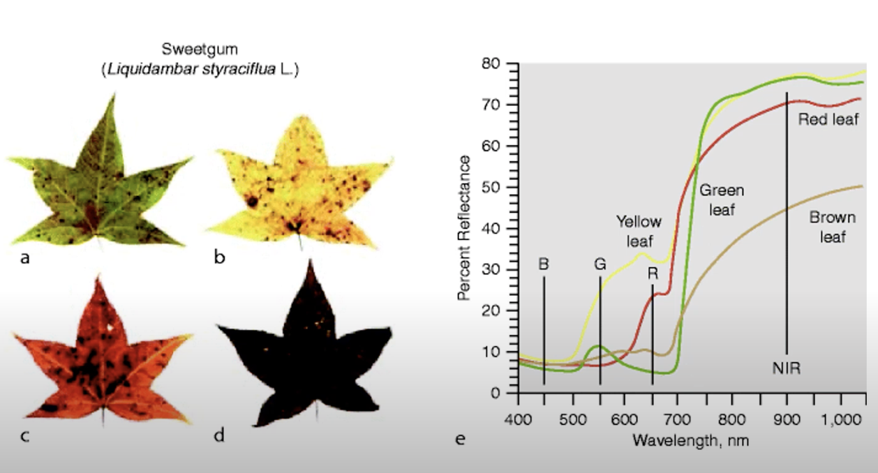
A road made of asphalt reflects sunlight in the visible spectrum almost evenly. Vegetation, in contrast, absorbs most blue and red light for photosynthesis, hence it appears green to the human eye, while reflecting NIR (800– 1,000 nm) radiation.
Stressed vegetation shows less absorption of red radiation (less chlorophyll) and a decrease in the NIR reflectance due to the leaf cell structure breaking down.
Remote sensing sensors can be divided into two main groups: active and passive.
Active Remote Sensing: Illumination of the Earth artificially by actively emitting and receiving radiation in the form of radio waves (RADAR; wavelengths ranging from 3 to 24 cm) or laser pulses (Light Detection and Ranging (LiDAR); typically, in the NIR wavelengths).
Passive Remote Sensing: Recording and analyzing reflected sunlight. In addition to radiation from the sun, some passive sensors also record thermal radiation that is emitted from the Earth’s surface (TIR).
Multispectral Sensors: Record 4-10 Bands and include Landsat, SPOT, and ASTER with 30m spatial resolution.
Hyperspectral Sensors: Record >100 narrow bands.
Spectral Sensors (imagers):
Advanced Spaceborne Thermal Emission and Reflection Radiometer (ASTER)
Enhanced Thematic Mapper Plus (ETM+)
IKONOS: Provides sub-meter spatial resolution.
MODerate-resolution Imaging Spectroradiometer (MODIS): SRS aboard the Terra and Aqua Satellites.
Multispectral Scanner System (MSS)
Operational Land Imager (OLI)
QuickBird: Provides sub-meter spatial resolution.
Satellite Pour l’Observation de la Terre (SPOT)
Worldview: Provides sub-meter spatial resolution.
Raster: Consists of a regular grid of single cells (pixels) as fundamental units. A set of numbers stored in a rectangular matrix. A very common raster format is a GeoTIFF, with the suffix “.tiff” or “.tif”.
Vector: Any continuous shape; areas, lines, points.
Bands: Used for raster layers of the same satellite image, for example, band 3 of the Landsat 5 Thematic Mapper (TM) of the same scene.
Scene (aka Tile): A rectangle of data covering a specific area of the Earth.
SRS Resolution includes:
Spatial resolution (m): Refers to the size of the pixels.
Temporal resolution (days): Refers to how many days it takes until a given scene is recorded again. MODIS passes the same place on Earth once every 2 weeks, Landsat, monthly.
Spectral resolution (bands): Refers to the number of spectral bands.
Radiometric resolution (bit): Refers to the gradations of brightness that can be stored in a data set. Determines the number of unique values that can be stored by the sensor in a pixel. A detector of 8-bit radiometric resolution, for example, can store 256 unique values, that are all integer values between 0 and 255. If you are plotting such an image in greyscale, you will see a gradient from black (value 0) to white (value 255).
Thematic resolution (classes):
Vector File: A spatial extension of a spreadsheet where every row corresponds to a specific location and the columns store various fields of information about the points, either as numbers or characters. If you open any GIS software and a vector file you will be able to see a table with entries for each spatial location, the so-called attribute table.
.shp: Shapefile containing geometry data; points, lines, polygons.
.shx: Shapefile containing index positions.
.dbf: Database file; attributes for each shape are stored in dBase format.
.prj: Shapefile containing coordinates and projection.
.sbn: Shapfile containing a spatial index.
.sbx: similar to .sbn.
For every project, check your data first when you are using spatial data:
Load all data into your software program.
Check the projections of the data sets.
Check if all layers match, that is, have the same projection and are displayed on top of one another.
Reproject the layers if needed.
LS 5 Natural Color: Combine spectral bands three (red), two (green), one (blue) into a so-called true colour RGB composite image by mapping band 3 to the RED color of your screen, band 2 to GREEN and band 1 to BLUE.
LS 5 Vegetation Symbology: Bands 4-3-2. This combination highlights the differences between vegetation and no vegetation. Vegetation appears red (coniferous trees are darker than broadleaved trees), grasslands are pinkish and urban areas with sparse vegetation tend to be blueish.
_____________________________________________________________________________
Chapter 3: Where to Obtain Spatial Data?
DL the vector outline of Brazil: (raster) brazil <- getData("GADM", country = "BRA", level = 1) plot(brazil)
DL precipitation data from WorldClim (http://worldclim.org/). These are global climate layers with a spatial resolution of approximately 1 km and available for download at a 0.5, 2.5, 5 or 10 degree spatial resolution: prec <- getData("worldclim", var = "prec", res = 2.5) names(prec) <- c("Jan", "Feb", "Mar", "Apr", "May", "June", "July", "Aug", "Sept", "Oct", "Nov", "Dec").
The naming convention for Landsat imagery (LXSPPPRRRYYYYDDDGSIVV) indicates all necessary information about a data set; L = Landsat; X = Sensor; S = Satellite; PPP = WRS path; RRR = WRS row; YYYY = Year; DDD = Julian day of year; GSI = Ground station identifier; VV = Archive version number (optional).
_____________________________________________________________________________
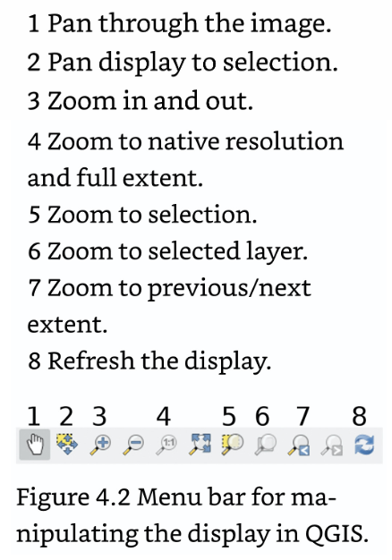
Chapter 4: Spatial Data Analysis for Ecologists: First Steps
The very first two things you should always do when you receive new spatial data are:
Display your data.
Check the projection.
Importing Field Data: Organize your coordinate pairs in a spreadsheet format with one row per coordinate pair, and your corresponding measurements which you would like to convert to a spatial data set. Then use the import .csv function in QGIS to import delimited text files. Specify the projection and save it as an ESRI Shapefile prior to closing.
On- Screen Digitization: Manual generation of new vector layers including digitizing features from a scanned geological map, deriving manmade features from satellite imagery including roads and waterways.
Importing Raster Data in R
Use the raster package to import and handle raster files in R.
raster(): Used for a single raster layer.
brick(): Used for multiple layers from a single file (i.e. GeoTIFF).
stack(): Used for separate files.
Importing Landsat Imagery (Example)
LS data are delivered in a separate GeoTIFF file for each band.
Command for loading a single band:
p224r63_2011_B1 <- raster("raster_data/LT52240632011210/LT52240632011210CUB01_B1.TIF")
To import all the layers, we could load each band separately and then use the stack() command
tmp1 <- raster("raster_data/LT52240632011210/LT52240632011210CUB01_B1.TIF")
tmp2 <- raster("raster_data/LT52240632011210/LT52240632011210CUB01_B2.TIF")
tmp3 <- raster("raster_data/LT52240632011210/LT52240632011210CUB01_B3.TIF")
p224r63_2011 <- stack(tmp1, tmp2, tmp3)
Since this is time-consuming, simply list all files matching a given pattern and load them in one go with stack(), which can take a list of file paths as input:
allBands <- list.files("raster_data/LT52240632011210/", pattern = "TIF", full.names = TRUE)
Now that all bands are in a single RasterStack, save it to a single multi-band GeoTIFF file on hard disk:
writeRaster(p224r63_2011, filename = "raster_data/LT52240632011210.tif")
Use rgdal::readGDAL() to directly import raster data into these classes.
writeRaster(): Saves raster data to disk in signed 8-byte float (FLT8S) data type.
Importing Vector Data
To represent spatial vector data in R, use the sp package. The primary object classes are SpatialPoints, SpatialLines and SpatialPolygons objects, which store the projection and coordinates of points, lines and polygons, respectively.
rgdal::readOGR(): supports almost any relevant file format, imports directly into the Spatial classes of the sp package and does a good job at importing projections.
Importing GPS Data
gpsPoints <- readOGR(dsn = "vector_data/field_measurements.gpx", layer = "waypoints")
Importing Field/CSV Data (Example)
Excel style field data can be loaded into R and converted to a spatial object afterwards. First, load the .csv file and take a look at it. The file has four rows (points), two columns of X and Y coordinates and further information, such as the name and measurements associated with each point:
csv_file <- read.csv("vector_data/csv_file_locationdata.csv") csv_file #> X Y id plot_name value #> 1 616528.0 -491023.9 1 NameOne 44.87 #> 2 627313.6 -496776.2 2 NameTwo 12.22 #> 3 627509.7 -504620.3 3 NameThree 99.01 #> 4 637903.1 -508542.3 4 NameFour 3.89
Next, convert this object into a SpatialPoints object:
csv.sp <- SpatialPoints(coords = csv_file[, c("X", "Y")]) csv.sp #> class : SpatialPoints #> features : 4 #> extent : 616528, 637903.1, -508542.3, -491023.9 (xmin, xmax, ymin, ymax) #> coord. ref. : NA
Finally, build a SpatialPointsDataFrame that holds the data values in columns 3–5 in an attribute table:
csv.spdf <- SpatialPointsDataFrame(csv_file[, c("X", "Y")], data = csv_file[3:5]) csv.spdf #> class : SpatialPointsDataFrame #> features : 4 #> extent : 616528, 637903.1, -508542.3, -491023.9 (xmin, xmax, ymin, ymax) #> coord. ref. : NA #> variables : 3 #> names : id, plot_name, value #> min values : 1, NameFour, 12.22 #> max values : 4, NameTwo, 99.01
A shortcut to transform a data.frame into a SpatialPointsDataFrame is to use the coordinates() function and specify the coordinate columns directly. Our csv_file is a "data.frame": class(csv_file) #> [1] "data.frame"
To get and set projections of spatial objects, use:
raster::projection(): projection(csv.spdf) <- projection(p224r63_2011)
Exporting Vector Data
Store your Spatial objects just like any other R object with save(), dump() or saveRDS().
writeOGR(): Saves SpatialPointsDataFrame files:
writeOGR(csv.spdf, "vector_data/processed/", "csv_spdf_as_shp", driver = "ESRI Shapefile")
writeOGR() function for exporting vector data to KML:
writeOGR(gpsPoints, dsn = "vector_data/processed/gpsPoints_GE.kml", layer = "myLayername", driver = "KML")
Plotting Spatial Data in R
plot(): Plots Raster Data in R.
Plot all bands separately: plot(p224r63_2011)
Plot only the fifth layer: plot(p224r63_2011, 5)
Change the colour palette: plot(p224r63_2011, 5, col = grey.colors(100))
Set layer transparency to 50%: plot(p224r63_2011, 5, alpha = 0.5)
raster::plotRGB(): Assigns and plots bands to a LS 5 TM Scene Example:
True Color: plotRGB(p224r63_2011, r = 3, g = 2, b = 1, scale = 1)
False Color (vegetation): plotRGB(p224r63_2011, r = 4, g = 3, b = 2, stretch = "lin")
geom_point(): Plots points.
geom_path() or geom_polygon(): Plots Polygons.
geom_path(): Plots lines.
geom_raster() or annotation_raster() or geom_tile(): Plots rasters.
geom_map() or coord_map(): Plots projected data with appropriate CRS.
CRS and Data Projection
Checking and ensuring spatial fit and conformity of projections should be one of your top priorities when you assemble data for a new project.
QGIS offer “on the fly” reprojection, which means they reproject all loaded data sets automatically to the current projection of your project (only for display; it does not modify the data permanently).
Projections and coordinate reference systems deal with the question of how to transform coordinates on a sphere – the Earth – onto a two-dimensional map by a mathematical coordinate transformation
Reprojecting Vector Data
Reprojecting Vector Data in QGIS: First, set the projection to the one of the raster by right-clicking on the raster entry and selecting “Set Project CRS from layer”, then save the vector file and tell QGIS to save and reproject it to the project projection.
Reprojecting Vector Data in R: First check the projection of the vector files:
projection(pa) #> [1] "+proj=longlat +datum=WGS84 +no_defs +ellps=WGS84 +towgs84=0,0,0"
projection(roads) #> [1] "+proj=utm +zone=22 +south +datum=WGS84 +units=m +no_defs +ellps=W GS84 +towgs84=0,0,0"
projection(csv.spdf) #> [1] "+proj=utm +zone=22 +datum=WGS84 +units=m +no_defs +ellps=WGS84 +tow gs84=0,0,0"
Reproject the pa vector to the same projection as the road vector using the spTransform() command.
raster::crs(), which is short for projection(…, asText = FALSE) to extract it from the roads object: pa_utmS <- spTransform(pa, CRS = crs(roads))
Reprojecting Raster Data
When reprojecting raster data, the new pixel locations might not be in a rectangular grid anymore after reprojecting but are instead forced to fit into a different grid orientation. Therefore, reprojecting rasters with any resampling method other than nearest neighbour is not reversible. Always opt for reprojecting the vector over the raster.
Reprojecting Raster Data in QGIS: Simply save the raster file to your file system with a new name.
Reprojecting Raster Data In R: Use the raster::projectRaster() function to warp, that is reproject and resample, a scene to another projection. The spTranform() function works for vector data only.
Raster–Vector Conversions
rasterize() command: Requires the vector layer as an input and a template raster with the target resolution and extent used to create the new raster.
pa_utmN_rast <- rasterize(pa_utmN, p224r63_2011, field = "wdpaid")
rasterToPolygons() and rasterToPoints() commands: Allows for raster data vectorization.
rasterToContour(): Creates isolines, typically from a DEM.
dem <- raster("raster_data/dem/srtm_dem.tif") contourLines <- rasterToContour(dem, levels = seq(50, 350, 50))
Spatial Queries: Extracting Values
ptVals <- p224r63_2011[csv.spdf]: Extracts values for rasters. You can also use raster::extract().
sp::over(): Extracting Values for Vectors.
Computing Distances and Buffers
raster::distance() command: Calculates a continuous distance field.
csv.spdf_dist <- distanceFromPoints(p224r63_2011, csv.spdf)
raster::pointDistance() command: Calculates the pairwise distance matrix between spatial points either in spherical (lonlat = TRUE) or planar coordinates (lonlat = FALSE).
Raster Processing: Cropping and Masking
crop() command: Crops Raster Data in R.
Cropping Raster Data in QGIS: Raster data can be cropped and masked using the “Clip raster by extent” and “Clip raster by mask layer” commands within the GDAL/OGR “Extraction” functions in the “Processing Toolbox”. Alternately, use Raster > Extract > Clipper.
Raster Arithmetic
The raster package provides arithmetic operations for direct use such as +, -, * and / on a per raster basis.
Adding two raster in R: b1b2sum <- p224r63_2011[[1]] + p224r63_2011[[2]]
To create a new raster holding the sum of all pixels from a RasterStack we can use sum():
totalSum <- sum(p224r63_2011)
Raster functions are mean(), log(), sqrt(), cumsum() or sign().
raster::calc() function: Main command for performing raster functions.
summary() command: Summarizes each layers values.
Managing Spatial Resolution
Decreasing the spatial resolution of a raster is accomplished by aggregating the values of neighbouring pixels and assigning them to a new pixel of coarser resolution. To do this use raster::aggregate() and aggregate our Landsat scene by a factor 2 from a 30-m resolution to a 60-m resolution. p224r63_2011_agg <- aggregate(p224r63_2011, fact = 2, fun = mean) res(p224r63_2011_agg) #> [1] 60 60
Raster Tricks
Orthorectification: Terrain-induced geometric distortions.
Optical remote sensing data are typically classified into successive processing levels.
Level 0: Raw data without any calibration or correction.
Level 1A: Raw data bundled with radiometric and geometric calibration and correction coefficients as well as geolocation information.
Level 1B: Level 1A data that has been georeferenced- each pixel corresponds to an explicit location on Earth.
Level 2: Geophysical parameters, such as reflectance at the Earth’s surface, land surface temperature or soil moisture, have been completed.
Reading Landsat Data in R: Landsat meta-data is stored in a plain text file ending in MTL.txt, which can be opened with any text editor software. Instead of reading the parameters manually from the text file, import it into R using readLines() (or XML::xmlParse() for XML files). You can also use RStoolbox::readMeta() which is explicitly designed to read Landsat meta-data:
library(RStoolbox) meta2011 <- readMeta("raster_data/LT52240632011210/LT52240632011210CUB01_ MTL.txt")
summary(meta2011) #> Scene: LT52240632011210CUB01 #> Satellite: LANDSAT5 #> Sensor: TM #> Date: 2011-07-29 #> Path/Row: 224/63 #> Projection: +proj=utm +zone=22 +units=m +datum=WGS84
_____________________________________________________________________________
Chapter 5: Pre-processing Remote Sensing Data
Radiation emitted from the sun reaches the Earth’s atmosphere relatively unaltered. However, as it travels through the atmosphere, it is scattered and absorbed by atmospheric gases and aerosols; this substantially changes the radiation spectrum. Once solar radiation is reflected from the surface it has to pass through the atmosphere a second time before it reaches the sensor.
Solar-Reflective Range: ~ 300 to 2,500 nm
Atmospheric Correction: Process of removing atmospheric effects from SRS.
Cloud Cover: A typical property distinguishing clouds from land surface is very low thermal radiation (clouds in high altitude are cold) and high reflectance in the visible region of the spectrum.
RStoolbox::cloudMask(): Identifies cloud pixels. This function calculates a spectral index between the thermal and blue bands ((thermal - blue) / (thermal + blue)) and applies thresholds to flag clouds.
RStoolbox::maskCloudShadow() function: Masks Cloud Shadows
Haze Removal (aka Dark Object Subrtraction- DOS): Based on the idea that there are always a few pixels that reflect almost no radiation (about 1% reflectivity is assumed) and hence should be dark.
RStoolbox::estimateHaze(): Estimates Haze Value on the DN data by specifying the proportion of dark pixels we expect in the image (darkProp).
Geolocation: Use of location technologies including GPS and IP to identify and track.
Topographic Illumination Correction
Panchromatic Band Sharpening: Use of Panchromatic (Pan) Bands with 15m resolution to enhance medium-resolution imagery. The idea of pan-sharpening is to substitute the medium-resolution spectral band’s brightness values with those of the panchromatic image. As a result we have a multispectral image at much higher spatial and spectral resolution. Use the RStoolbox::panSharpen(): Pan Sharpening.
_____________________________________________________________________________
Chapter 6: Field Data for Remote Sensing Data Analysis
Selecting Sample Size: When using satellite data with a 1,000 m spatial resolution, the best approach would be to set sampling points in each of the 1,000 × 1,000 m grid cells to have a representative sample for each pixel and to collect information across several pixels. Finer-scale sampling might not be needed because the remote sensing data will only provide you with one value for each 1,000 × 1,000 m grid cell.
Field Sampling Time: Field sampling should be linked to Earth Observation data and take place at the same time as remote sensing data acquisition. Moreover, a cloud-free period is recommended as optical sensors cannot record land surface conditions under clouds.
Sampling Techniques
Simple Random Sampling: The least biased sampling technique- all parts of the study area have an equal chance of being selected.
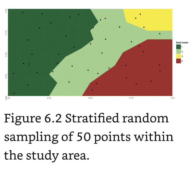
Stratified Random Sampling: Useful when a priori knowledge of the landscape exists to develop subsets of the entire landscape.
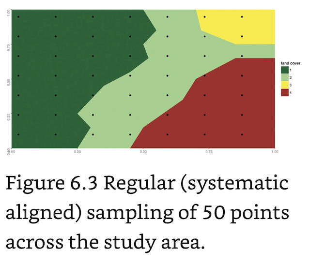
Regular (or systematic aligned) Sampling: Samples are evenly distributed at equidistant intervals throughout the region of interest.
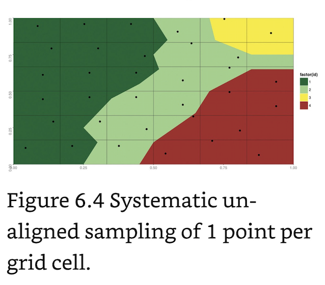
Systematic Unaligned Sampling: Random sampling of units within each grid cell.
Cluster sampling:
Sampling in R
sp package: Used for spatial sampling.
spsample() function: Sample point locations within a spatial object (square, grid, polygon, spatial line, circle) with different sample patterns (random, regular, stratified, non-aligned, hexagonal, clustered, Fibonacci). R Command to sample 100 random points:
set.seed(1) RandomPoints <- spsample(x = SpatialObject, n = 100, type = "random")
Three main arguments must be defined. The first argument x is a spatial object (for example, grid, line or polygon). The second argument n gives us the number of samples and with type we specify the sampling pattern (here: "random"). In this example we sampled 100 random spatial points within our bounding box (the SpatialObject). The spsample() function returns a SpatialPoints object with X and Y coordinates.
randomSample() command: Samples random points on top of a raster file.
_____________________________________________________________________________
Chapter 7: From Spectral to Ecological Information
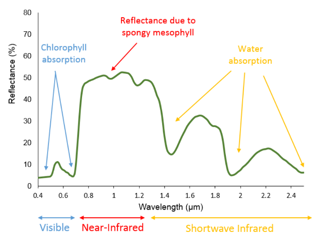
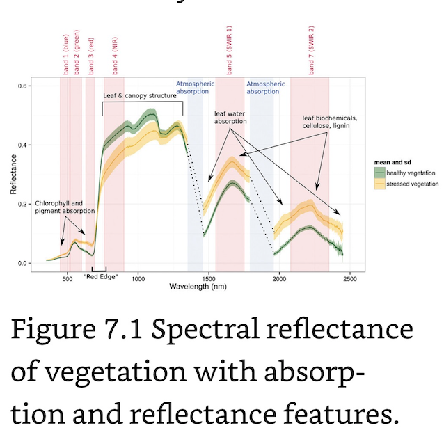
Physical states such as photosynthetic activity, water stress, leaf biochemical constituents and so on all contribute to shape the reflected spectral signal. In regard to vegetation, the most important wavelengths of a Landsat image are the red and NIR regions, which are used as proxies for the photosynthetic health and activity of vegetation.
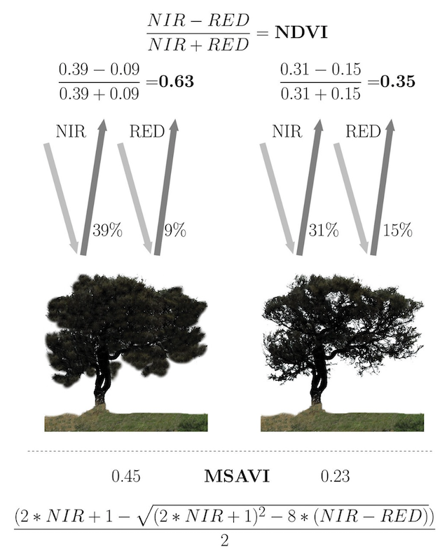
Healthy vegetation exhibits very low reflectance in the red region, due to photosynthetic absorption of light and very high reflectance in the NIR due to scattering processes at the leaf level. With decreasing photosynthetic activity, the difference between red and NIR will decrease, and the red to NIR ratio flattens. The characterization of this contrast, the so-called “red edge”, is the foundation of many VI’s.
Vegetation indices (VIs): Used as physically interpretable predictors in land cover change analysis, species distribution modelling and the spatial resource use of animals, among many others.
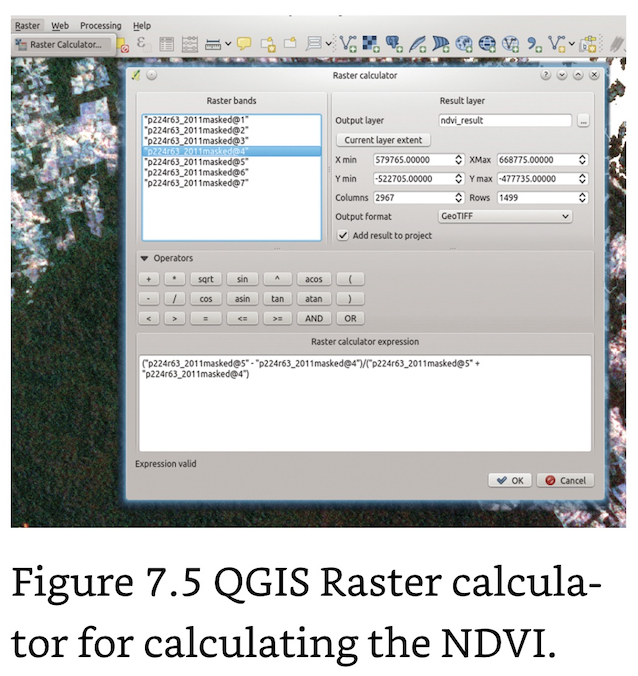
Normalized Difference Vegetation Index (NDVI): Linked to vegetation cover, biomass and thus net primary productivity. The values of the NDVI (and many other indices) range from -1 to +1, with higher values indicating higher differences in the red edge and hence higher photosynthetic activity or vegetation greenness. Values near 0 are usually non-vegetated areas and negative values usually indicate water.
NDVI in R: Load Landsat scenes from 1988 and 2011:
p224r63_2011 <- brick("raster_data/final/p224r63_2011.grd")
p224r63_2011m <- brick("raster_data/final/p224r63_2011_masked.grd")
p224r63_1988m <- brick("raster_data/final/p224r63_1988_masked.grd")
The NDVI function has the two input layers as arguments (nir, red), which are entered into the formula within curly brackets: ndvi_formula <- function(nir, red) { (nir - red)/(nir + red) }
Normalized Difference Water Index (NDWI)
Triangular Vegetation Index (TVI)
Modified Soil-adjusted Vegetation Index (MSAVI2)
_____________________________________________________________________________
Chapter 8: Land Cover & Image Classification Approaches
Land Cover Classification: Conversion of multiple input layers to groups of pixels with similar characteristics. Resulting pixel values are used to identify different land cover classes that are either defined a priori (supervised classification) or with a clustering algorithm (unsupervised classification).
Image Classification Steps
1. Define why you want a classified image and how you will use it.
2. Define the study area.
3. Select/develop a classification scheme (define classes).
Classification Scheme: Defines classes to be delineated, the map’s legend. Too many classes will reduce the per-class accuracy and too few might result in mixed classes and a reduction in the usefulness of the map.
Minimum Mapping Unit (MMU): The minimum area that a group of pixels of a single class must have.
4. Select the imagery (resolution, sensor, date).
VHR imagery, such as 0.5 m WorldView-2 imagery.
Texture: Calculated by determining the variability of pixel values in a neighborhood around a center pixel.
5. Prepare the imagery for classification (image corrections, subsetting).
6. Collect or generate ancillary data (VIs, texture).
7. Choose a classification approach (supervised, unsupervised). A common method is to do the classification using automated methods and then manually edit the resulting classified image with editing techniques to effectively correct errors that can be identified after visual inspection of the map.
Supervised: Technique used for the quantitative analysis of SRS using labeled input.
Unsupervised: Identifies clusters of similar pixels automatically and it is up to the user to make sense out of these classes. Popular unsupervised approaches are kmeans, ISODATA and hierarchical clustering.
Cluster-Busting: Labeling the classes that are well classified and then running another unsupervised classification using only those pixels that were not well classified. The process is repeated until the entire image is classified.
kmeans: An algorithm that find clusters of minimal within-cluster variance.
Random Forest
Partial Least Squares Regression (PLSR)
Support Vector Machines with a radial basis kernel (SVM)
8. Collect training and validation data.
9. Create a classification map (modelling): enter your image data (predictor variables) and training data (response variable) into the algorithm and let it go to work.
10. Assess classification accuracy and refine, if necessary.
Typically, we would use roughly 70% of the data for training and 30% for validation.
Errors in a classified map occur either because the object (a pixel or an image segment) being classified was assigned the wrong class label, due to confusion with another class, due to the landcover class not being part of the legend, or because the location of the object on the map is not accurate.
Planning an accuracy assessment involves three steps: 1 develop a sample design; 2 collect and compile validation data; 3 calculate accuracy statistics and check consistency visually.
Accuracy Metrics
Confusion Matrix (aka Contingency Table): Standard methodology to calculate accuracy metrics of a classification. It contrasts the actual, observed or “true” class of a sample (from fieldwork or image interpretation, sometimes referred to as ground truth) with the class predicted by the model for each validation pixel.
Overall Accuracy
Producer’s accuracy (aka Sensitivity): Accuracy from the perspective of the map producer (How well does my model recognize a class?) and is calculated as the proportion of correctly classified pixels per class.
User’s accuracy (aka Positive Prediction Value): Assesses accuracy from the perspective of the map user (What is the probability that a pixel predicted as forest is actually forest?). It is calculated as the number of correct predictions relative to the total number of times a class was predicted.
_____________________________________________________________________________
Chapter 9: Land Cover Change or Change Detection
Raster Calculator Subtraction: The most straight forward method to calculate change between two images is simply taking their difference- subtract the later year NDVI from the earlier.
Spectral Change Vectors: Calculates transformation bands for scenes (i.e. Landsat). Change vector magnitude is calculated as the Euclidean distance between two corresponding pixels in a 2D space spanned by the brightness and greenness bands.
Use the RStoolbox::rasterCVA() for the calculation: changeVec <- rasterCVA(tc2011[[1:2]], tc1988[[1:2]])
Multi-Date Classification: Relies on direct change classes without any previous single classification. Combines all bands from two scenes from different dates into a stack with, for example, 10 bands (first 5 Landsat bands of each time step) and is fed into a classification trained by vector data on changed areas.
fractional cover (fCover) analysis (aka %cover or continuous fields): Derives fractional cover for a subset of the study area, model the statistical relationship between fractional cover and spectral reflectance and finally to predict the fractional cover of each class based on the spectral reflectance of a coarser resolution image of a bigger extent
_____________________________________________________________________________
Chapter 10: Continuous Land Cover Information
Calculating fCover (aka Image Regression)
Acquire two images from the same region and with the same date.
One image should have a much finer resolution than the other, for example, Worldview-2 (2.5 m) and Landsat (30 m) or Landsat (30 m) and MODIS (250 m). The finer-resolution image will be used to create training data and the coarser-resolution image will be used to create the continuous fields layers. It is not necessary for the high-resolution image to completely cover the area of the coarser-resolution image, because areas outside of the overlap will be predicted by the model.
Carry out a land cover classification of the higher-resolution image using the classes for your fraction of vegetation cover (fCover) analysis (for example, forest, grass, water).
Use the higher-resolution image to calculate the % coverage for each of the cover types of interest, at the resolution of the coarser-resolution image. This results in a percentage cover raster layer at the coarse resolution for each of your cover types of interest. Summed up over all classes you should get a total of 100% for each pixel.
Fit the model by regressing the fCover values against the bands of the coarse resolution imagery.
Apply the model to the complete coarse resolution image and predict the fCover of each class.
_____________________________________________________________________________
Chapter 11: Time Series Analysis
Time Series Analysis: Explains how to use time series data provided by MODIS for deforestation monitoring. Landsat or AVHRR time series could also be used and might lead to other results due to their spatial resolution or temporal coverage. MODIS data come only in 250 m spatial resolution
Remote Sensing Time Series: A collection of repeated observations from a specific region.
Land Surface Phenology: The study of the spatio-temporal development of vegetated land surfaces in relation to climate by SRS.
Change Detection and Temporal Analysis
Find a MODIS Tile overlapping your study area: http://gis.cri.fmach.it/modis-sinusoidal-gis-files
Install the MODIS Package in R: install.packages("MODIS", repos = "http://R-Forge.R-project.org") library(MODIS)
To detect change, apply a pixel-based time series method, bfastmonitor, available in the BFAST R package (http://bfast.r-forge.rproject.org).
_____________________________________________________________________________
Chapter 12: Spatial Land Cover Pattern Analysis
Texture Analysis: Analysis of local spatial variability. Aims to derive so-called special texture metrics, which are indicators of how variable the environment of a given pixel is.
Moving Window Operation: Uses surrounding pixels to calculate statistical variability.
Filtering: Smooths data by removing unwanted noise. The simplest smoother is the mean. Calculate it either by specifying the function mean() in the execution of the focal() command, or by adjusting the weights matrix.
Landscape Fragmentation Analysis: Similar to texture analysis and relevant for ecological studies.
_____________________________________________________________________________
Chapter 13: Modeling Species Distributions
Species distribution models (SDMs): Link data on the distribution of species to environmental conditions, such as climate or land cover information. The two main aims of SDMs are prediction and understanding in order to guide conservation decisions including managing biological invasions, identifying and protecting critical habitats, selecting reserves, and translocation.
SDM Prediction: Where to look for a species and where to protect it.
SDM Understanding: What are the main factors determining species distribution and what is the effect of a disturbance, such as a road?
SDM Process
1. Formulate the Problem.
2. Collect Data.
3. Data Pre-Processing:
Combine Species Data and Environmental Information.
Data visualization.
Inspect Data for Collinearity- correlation between environment and variables.
4. Modeling: the species is modelled as a function of five environmental predictors:
The fCover in the particular cell (0 or 1).
The fraction of fCover in a 1,000 m radius surrounding the cell (0–1).
The distance to a PA (scaled from 0 to 1, where 1 represents 5,000 m or more).
NDVI (0–1).
The variance of the elevation in a 3 × 3 moving window around the cell.
5. Interpretation.
6. Process Iteration
Predict the probability of occurrence of the virtual species for each grid cell in the landscape with the function predict() from the raster package.
rfmap <- predict(p224r63_2011, rfmodel, type = "prob", index = 2)
_____________________________________________________________________________
Chapter 14: Introduction to the Added Value of Animal Movement Analysis and Remote Sensing
Methods for collecting animal movement data:
Lagrangian Method: Position is communicated at regular time intervals; radio-tracking, satellite tracking, GPS, geolocators, rings and bands.
Eulerian Method: Multiple locations are continuously surveyed and individuals within reach of observation locations are identified; camera traps, RFIDs, Mic arrays, video surveys.
Movement Data Analysis:
1. Data Inspection
Usually, tracking data comes as a .csv file that can be opened in R:
R Code: move_csv <- read.csv("vector_data/move_data.csv", as.is = TRUE)
Next, convert the data frame into a spatial object. Since the tracking data are point observations an appropriate class is a SpatialPointsDataFrame.
R Code: coordinates(move_sp) <- c("y", "y") projection(move_sp) <- projection(p224r63_2011m)
2. Data Visualization
3. Data Cleaning: Removal of temporal and spatial outliers.
4. Data overview with summary statistics.
_____________________________________________________________________________
Terminology & Acronyms
Akaike Information Criterion (AIC): Widely used criterion to make the decision whether to keep a variable. Models with lower AIC will have a better predictive performance on future data.
Bands: Used for raster layers of the same satellite image, for example, band 3 of the Landsat 5 Thematic Mapper (TM) of the same scene.
Bilinear Resampling: Calculates a distance-weighted average from the four closest pixels relative to the new central pixel.
Brownian Bridge Movement Model (BBMM): A method of quantifying the distribution of an animal accounting for errors in temporal sequence and location. Its extension, the dynamic Brownian bridge movement model (dBBMM), accounts for additional changes in the behavior and thus the underlying movement process.
Collinearity: High correlation between variables. A commonly used value for a “high” correlation is 0.7.
Contextual Domain: Sets the spatio-temporal analyses of the first two domains in an environmental or physiological context and is the ultimate purpose in many ecological and conservation questions.
Coordinate Reference System (CRS)
Coregistration: The Spatial alignment of a series of images.
Corridors: Strips of native vegetation or habitat connecting otherwise isolated remnants.
Digital Elevation Model (DEM): Elevational Data.
Environmental Systems Research Institute (ESRI)
Geographic Information Systems (GIS): Spatial data handling and analysis using software.
GPS Exchange Format (GPX)
Histogram Matching: Matches the contrast of two images.
Home Range: The area traversed by an individual animal in its normal activities of food gathering, mating and caring for its young.
Image Segmentation: The process of grouping neighboring pixels into segments or objects, for example tree crowns or forest patches, which are then used as entities instead of pixels.
Intensity/Hue/Saturation (IHS)
Invasive Alien Species: Introduced species whose introduction does or is likely to cause economic or environmental harm or harm to human, animal or plant health.
Minimum Convex Polygon (MCP) Method: Measure for describing a home range from positional data. In R, it can be calculated with the adehabitatHR package: library(adehabitatHR).
No Free Lunch Theorem: Testing different theorems and choosing the best one for your problem at hand.
Protected Area (PA)
R: A language and environment for statistical computing and graphics with a large number of extensions called packages (http://cran.r-project.org/web/packages/).
Raster: Consists of a regular grid of single cells (pixels) as fundamental units. A set of numbers stored in a rectangular matrix. A very common raster format is a GeoTIFF, with the suffix “.tiff” or “.tif”.
Reducing Emissions from Deforestation and Forest Degradation (REDD)
Remote Sensing: The acquisition of info about the Earth’s surface without being in physical contact with it.
RStudio: The most popular IDE for R (http://www.rstudio.com)
Scene (aka Tile): A rectangle of data covering a specific area of the Earth.
Spatial Bookmarks Feature: Allows you to bookmark a view of a certain zoom level and location.
Satellite Remote Sensing (SRS)
Utilization Distribution (UD) Model: Presents an animal track or location as a 2D probability distribution. The UD corresponds to an animal’s relative frequency of occurrence; hence, it is the probability of finding an animal in a defined area within its home range.
Vector: Any continuous shape; areas, lines, points.
Worldwide Reference System (WRS-1 or -2)
_____________________________________________________________________________
Resources
Animal Movement and Remote Sensing for Conservation (AniMove): http://animove.org
Animal Tracking Database Movebank: https://www.movebank.org/
Applications of R: http://www.cran.r-project.org/manuals.html
Biodiversity Informatics: http://www.amnh.org/our-research/center-for-biodiversity-conservation/biodiversity-informatics
Change Detection on SRS Image Time Series: https://dutri001.github.io/bfastSpatial
Defense Meteorological Satellite Program (DMSP): http://ngdc.noaa.gov/eog/dmsp.html
EarthExplorer: http://earthexplorer.usgs.gov/
Earth Observation community (CEOS Biodiversity): http://remote-sensing-biodiversity.org/networks/ceos-biodiversity
Earth Observing System Data and Information System: http://reverb.echo.nasa.gov/reverb
ESA Sentinel Data Hub: https://scihub.esa.int/
Fraction of Green Vegetation Cover (Copernicus): http://land.copernicus.eu/global/?q=products/fCover
GIS File Info Website: http://www.fileinfo.com/filetypes/gis
GIS Instructional Guide: http://book.ecosens.org
GEO Biodiversity Observation Network: http://geobon.org
Global Land Cover Facility Earth Science Data Interface (ESDI): http://www.landcover.org/
Intro to R: http://cran.r-project.org/doc/contrib/Paradis-rdebuts_en.pdf
Landsat Ecosystem Disturbance Adaptive Processing System (LEDAPS): USGS provided atmospherically corrected Landsat Imagery to at-surface reflectance level.
Landsat Ecosystem Disturbance Adaptive Processing System (LEDAPS): USGS provided atmospherically corrected Landsat Imagery to at-surface reflectance level.
Landsat Tree Cover Continuous Field (Global Land Cover Facility): http://landcover.org/data/landsatTreecover
MODIS Land Vegetation Continuous Fields: http://modis-land.gsfc.nasa.gov/vcc.html
NOAA Climate Data: http://ropensci.org/tutorials/rnoaa_tutorial.html
Portal of the Brazilian Space Agency INPE: http://www.dgi.inpe.br/CDSR/
Project Projections: http://projectionwizard.org
QGIS Plugins:
GPStools: Importing and modifying GPS data.
fTools: Vector analysis and management.
OpenLayers Plugin: Display of Google Earth, OpenStreetMap, Bing Maps, etc.
Georeferencer GDAL: Georeference raster using GDAL.
Processing: interfaces to GRASS, OTB, R, SAGA.
R: A language and environment for statistical computing and graphics with a large number of extensions called packages (http://cran.r-project.org/web/packages/).
RStudio: The most popular IDE for R (http://www.rstudio.com). Another free option is Eclipse (http://www.eclipse.org), to be used with the Eclipse-based StatET plug-in (http://www.walware.de/goto/statet).
Raster Package: Turns R into a fully fledged GIS.
R Errors:
“function_name”: You have either misspelled the function or forgotten to load the package providing this function.
R Packages
biomod2 package: Species Distribution Modeling.
dismo package: SDM Tutorial
letsR package: Provides information on the geographic distribution of species and environmental variables based on the IUCN Red List of Threatened Species database.
MODIS package: Provides functions to download, analyze, and visualize MODIS data.
rgbif package: Retrieves species data including the Global Biodiversity Information Facility (GBIF).
sp package: Provides SRS functions such as Landsat data processing, land cover classification, and data sampling.
spectralIndices() package: Spectral Indices.
R Functions
ls_multiscene_m <- mosaic(p224r63_adjacent, p224r63_2011[[layers]], fun = mean)
radCor(): Converts the thermal bands to brightness temperature (in degrees Kelvin).
randomSample() command: Samples random points on top of a raster file.
raster::getData(): Allows you to query several freely available spatial data sets, for example from the Global Administrative (GADM) database (http://gadm.org/) and download the data into R. getData() can also be used to dl raster data including elevation and climate variables.
raster::merge(): Merges two or more scenes.
raster::mosaic(): Calculates an average pixel value for overlapping regions.
rebird: Retrieves bird species data.
spsample() function: Sample point locations within a spatial object (square, grid, polygon, spatial line, circle) with different sample patterns (random, regular, stratified, non-aligned, hexagonal, clustered, Fibonacci).
rgeos: Provides functions for complex GIS operations like buffering or intersecting vector data, and interfaces the external Geometry Engine – Open Source (GEOS) library.
rfishbase: Retrieves fish species data. rgdal: Provides functions for import and export of spatial data in a variety of formats, i.e. shapefile, Keyhole Markup Language (KML) or GeoTIFF and projection transformations.
rnoaa: Enables you to download NOAA climate data directly into R.
untar() function: Unzips files in R.
RStoolbox: Provides functions for remote sensing data analysis.
RStoolbox::cloudMask(): Identifies cloud pixels. This function calculates a spectral index between the thermal and blue bands ((thermal - blue) / (thermal + blue)) and applies thresholds to flag clouds.
RStoolbox::maskCloudShadow() function: Masks Cloud Shadows
RStoolbox::coregisterImages(): Coregisters two scenes.
RStoolbox::estimateHaze(): Estimates Haze Value on the DN data by specifying the proportion of dark pixels we expect in the image (darkProp).
RStoolbox::histMatch(): Histogram Matcher, matches the contrast of two images.
p224r63_adjacent_hm <- histMatch(p224r63_adjacent, p224r63_2011[[layers]]) Then, we merge them into one mosaic: ls_multiscene_hm <- merge(p224r63_adjacent_hm, p224r63_2011[[layers]])
RStoolbox::panSharpen(): Pan Sharpening.
R-Related Training: http://www.r-project.org/doc/bib/Rbooks.html
Remote Sensing and GIS in Ecology & Conservation (EcoSense): http://ecosens.org
Remote Sensing Conservation network (CRSnet): http://remote-sensing-biodiversity.org/networks/crsnet
Remote Sensing for Biodiversity & Conservation: http://remote-sensing-biodiversity.org/resources/
RS-ecology: http://lists.uni-wuerzburg.de/mailman/listinfo/rs-ecology
Spatial Pattern Analysis Program for Categorical Maps (FRAGSTATS: http://www.umass.edu/landeco/research/fragstats/fragstats.html
Spatial References: http://spatialreference.org
Species Distribution Data: http://www.gbif.org/
Transforming Science through Open Data project: https://www.ropensci.org
Tree Cover Continuous Fields (Global Land Cover Facility): http://landcover.org/data/treecover
USGS Global Visualization Viewer: http://glovis.usgs.gov/
Visible Infrared Imaging Radiometer Suite (VIIRS): http://ngdc.noaa.gov/eog/viirs.html
_____________________________________________________________________________
Misc Quotes
“One of the Aichi biodiversity targets of the Convention on Biological Diversity is to conserve at least 17% of terrestrial and 10% of marine areas in equitably managed, ecologically representative and well-connected PAs by 2020.”
“Observable changes in atmospheric gas concentrations have translated into increased global surface temperature; shifts in seasonal climatic patterns; extreme climatic events becoming more frequent and occurring with greater intensity; glacier reduction; sea surface ice reduction; and increased sea levels. Wildlife is directly or indirectly responding to changes in these climatic patterns, with many studies reporting latitudinal and altitudinal distribution range shifts; migrant birds arriving earlier and starting to breed earlier; reduced survival or reproduction; and increased extinction risk.”
“Responses of species to climatic changes can be expected to fall into one of the following three categories: (1) thrive (that is, the species can live under the new set of environmental conditions); (2) adapt (that is, the species can change its ecology or distribution to avoid extinction); (3) go extinct (that is, the species will slowly decline and eventually be lost).”
“All models are wrong, but some are useful.”-George Box.
“One possible strategy to increase the effective size of populations, and make them more resilient to inbreeding, demographic stochasticity and the Allee effect is to include corridors in conservation plans so that connectivity between otherwise isolated patches of habitat is increased.”
_____________________________________________________________________________
Chronology
May, 2003: The ETM+ sensor of Landsat 7 satellite loses most of its usability due to a mechanic failure, resulting in ~22% data loss distributed across most of the scene in a striped pattern.-GIS by Wegmann.
2001: The MODerate-resolution Imaging Spectroradiometer (MODIS) is launched as part of the Terra and Aqua Satellites. Terra MODIS & AQUA MODIS have been viewing the entire Earth’s surface every 1- 2 days, acquiring data in 36 multispectral bands. The spatial resolution of the red and infrared band is 250 m (nadir), which makes it particularly suitable for studies on vegetation or land cover characterization through land cover classification.-GIS by Wegmann.
1988: The AVHRR/3, with six multispectral bands, is launched into Polar Orbit.-GIS by Wegmann.
1981: The AVHRR/2, equipped with six multispectral bands, is launched into polar orbit.-GIS by Wegmann.
1978: NOAA’s Advanced Very High-Resolution Radiometer (AVHRR) is launched into Polar Orbit aboard the TV IR Observation Satellite- N (TIROS-N). AVHRR measures the Earth’s reflectance in four multispectral bands.-GIS by Wegmann.
_____________________________________________________________________________